



IntelliPaper
Abstract
This paper studies DC micro-grids in mesh topology where voltage regulation is performed at each node with help of storage devices interfaced through boost converters. Loads and distributed power sources are treated as arbitrary perturbations under a hierarchical control strategy. The primary level controller is characterized by its faster actuation rate and focus on the implementation of distributed voltage sources, while the secondary level uses a consensus algorithm to reach power sharing among the sources, and introduces an auxiliary loop to secure voltage regulation around the nominal value. We model the entire network, considering the switching process of each individual converter, primary and secondary level controllers, hardware and communication interconnections, as a discrete time system, in opposi- tion to the documented continuous time dynamic assumption. This leads to obtain an explicit representation of the entire grid, which is closer to its final hardware implementation, and facilitates dynamic trajectory analysis over specialized or conventional hardware. The developed convergence criteria for the discrete time closed loop system is corroborated by dynamic simulations which also show the main benefits of the discrete time modeling.
Explore Digital Article Text
I. INTRODUCTION
DC microgrids are becoming increasingly important for integrating renewable energy sources into the power grid. By utilizing distributed generation units to meet local demand, these microgrids play a critical role in the transition towards a more sustainable energy matrix . What started as a simple photo voltaic (PV) microgrid implementation, as seen in , has evolved into complex mesh topologies with distributed generation units that require autonomous control to avoid centralized planning. This approach enhances the reliability and power quality of local users .
In the context of DC microgrids with smart actuation on distributed generation units, it is possible to adopt the hierarchical control schemes proposed for AC microgrids, as presented in . Various studies have reviewed this approach, including . At the primary level of control, electronic power sources are implemented with commutated circuits that exhibit small time constants, which have been studied in standard power electronics textbooks such as .
At a slower actuation rate, the secondary level of control in microgrids focuses on regulating entire microgrids with multiple active buses. Similar to multi-agent systems, each regulated voltage source must have a control unit to process signals received from other units or locally measured. This topic has been extensively documented in various sources, including books like . In DC microgrids, droop control is a popular strategy, as seen in . However, consensus-based approaches have also become important in achieving global control objectives such as power sharing , voltage regulation , and more recent approaches as presented in .
While most of the literature on microgrids uses idealized continuous time dynamics, in reality, power electronic sources and distributed controllers are implemented on digital hardware that runs on different clocks. Therefore, discrete time modeling of the individual components of a microgrid is necessary for closed-loop convergence analysis, making it more applicable to the final hardware implementation. As seen in various references, such as , hardware-in-the-loop technologies and real-time simulations using dedicated hardware can be further improved with accurate modeling of the control reality, especially when hierarchical primary and secondary level controllers have different actuation rates and communication dynamics that are implemented over multiple microcontroller platforms.
In this paper, we investigate DC micro-grids with a mesh topology and bi-directional boost converters as voltage sources, controlled under primary and secondary level strategies. Our goal is to develop discrete-time models for the various components of the control plant, both individually and as a whole. This includes the power electronic switching sources, distributed primary and secondary level controllers, and the hardware and communication interconnections between them.
Drawing from existing control strategies, we focus on implementing a primary level controller that utilizes an integral action function to interface with the secondary level. The secondary level control system implements a consensus algorithm to achieve power sharing and a novel auxiliary loop to achieve voltage regulation. We present necessary conditions for control gains to guarantee convergence of the secondary level closed loop system. As a result, we present a discrete time algorithm to compute the state trajectory, taking into account the actuation rates of the different control levels and non-ideal information exchange, which can be used for the partial implementation of the system on dedicated hardware.
After this introduction, Section 2 presents the micro-grid model and its components, focusing on the discrete-time digital solution of the differential equations. In Section 3, we describe the hierarchical control strategy for digital distributed hardware and provide necessary criteria for achieving power sharing and average voltage regulation under idealized conditions. In the subsequent section, we present the computational algorithm for the closed-loop system and provide a numerical example to verify the main characteristics of the closed-loop system and the simulation methodology.
Through this paper, matrix is the transpose of A and is its element in the i-th row and the j-th column. The identity matrix and the null matrix are respectively denoted by I and 0. A column vector of ones is denoted as 1, and a vector with zeros in every position except in the i-th row where its value is one, is denoted as so that .
II. MICRO-GRIDS IN MESH TOPOLOGY
2.1 Technological Description
Consider the two-node micro-grid illustrated in Figure 1. In this configuration, each node is equipped with a PV system, which consists of generation, conversion, and filtering stages. The PV system is designed to function as a current source, meaning that it does not regulate the voltage level at the
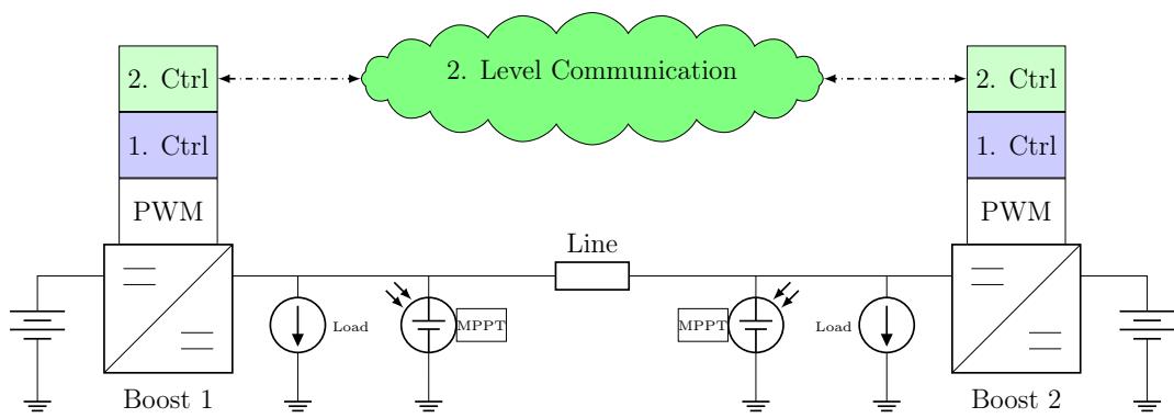
Figure 1: A two nodes example micro-grid
node. Instead, it strives to inject as much power as possible using a Maximum Power Point Tracker (MPPT) algorithm. Other types of distribution generation technologies could be modeled in a similar way. Likewise, the loads at each node can be modeled as a current source due to their unknown behavior, which may exhibit a time-variant ZIP characteristic. Since both the PV generation and load depend on unregulated external variables, they can be considered as perturbations.
To address the variability of PV generation, a storage device is connected to each node via a bidirectional DC/DC boost converter. The goal is to absorb excess power and inject it back into the system when load demand increases. These devices can be fully controlled and thus represent control actuators for voltage regulation at the nodes. Moreover, both nodes are connected to share generation and storage capacities, enabling the system to operate as a hardware-interconnected micro-grid instead of isolated nodes.
The standard approach to micro-grid control is a three-level hierarchy (e.g., [6, 8, 9]). At the primary level, the main objective is to implement individual voltage sources. This control layer can be physically implemented at each local unit without communication, relying on local measurements and actuation signals. Since the primary level plant involves fast dynamics, actuation should be performed at a high rate.
At the secondary level, control objectives are defined in terms of the entire micro-grid, rather than the individual distributed agents (i.e., the individual voltage sources serving as actuators for the secondary level process). Therefore, communication between different distributed controllers is mandatory for efficient functioning. The main goal at this level is to achieve predictable behavior of the micro-grid in terms of injected power and voltage levels, so
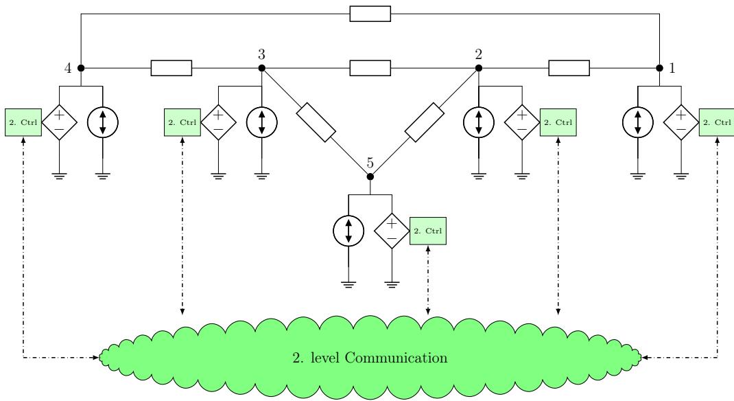
Figure 2: A five nodes example micro-grid
that the tertiary level control can rely on the fully functioning system. The higher level focuses on long-term energy exchange within the micro-grid or with respect to the main grid.
The basic idea of the two nodes micro-grid can be extended to larger system when more nodes are connected. This leads to the implementation of grids with possibly mesh-topologies as the five nodes example in Figure 2. Here, the boost converters that interface the storage devices and the primary control layer are drawn together as controllable voltage sources. The secondary layer follows the same distributed control philosophy as in the previous example. Note that the communication between the controllers is not necessarily dictated by the hardware links between the nodes. The parallel aggregation of different perturbations (loads and distributed generation) is represented by a double direction uncontrollable current source.
A micro-grid can be considered as a special case of a grid with mesh topology, in which the number of nodes, the geographical region, and the power ratings are restricted. In order to study such a reality, we need independent models of the hardware interconnections (the transmission or distribution lines) and the controllable voltage sources.
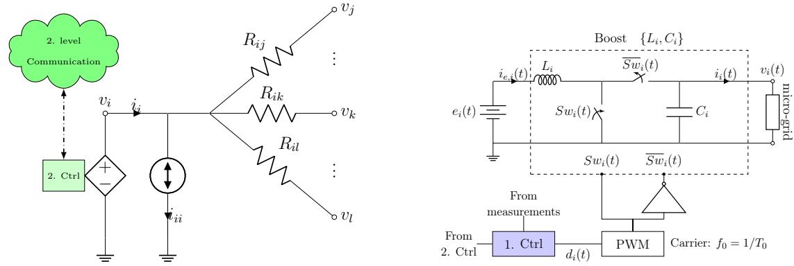
Figure 3: Voltage and current at node i of a mesh-grid with Figure 4: Ideal boost converter at the i-th node as a voltage source
2.2 Circuital Description
We will consider a mesh-grid as a graph , with N vertices or electric nodes , where DC voltage regulation can be performed and where loads and other generation units are connected. The undirected edges are transmission lines between the nodes, denoted . It is assumed that the grid is connected and therefore every active node has at least one neighbor node .
At every active node , we will consider that the uncontrollable current source models the aggregated behavior of all loads and distributed generators and consumes a net power . In this way, if , the injected power at the node surpasses the power consumed by the loads. In any case, this quantity is a disturbance as it depends on external uncontrolled variables as weather or consumption.
A transmission line between nodes i and will be assumed as a resistance because the effect of inductances can be neglected in steady state. The line parameters can be estimated with reasonable accuracy due to the small size of a micro-grid. A circuital representation of a node in the grid can be seen in Figure 3.
If is the current injected by a voltage source at node i, and is the node voltage, from Figure 3, an expression for the current as a function of the node voltages can be obtained:
with the net current consumed by the arbitrary loads. This expression can be generalized to all nodes by
where,
and such that its elements are given by
Because , coincides with the Laplacian matrix, denoted , of the undirected weighted graph , where the weight function is given by , for every edge . It is a well known fact that is a positive semi-definite matrix and that each row and column of sums up to zero. i.e. and .
2.3 Boost Based Actuators
At every node , an ideal bidirectional boost converter like in Figure 4 is implemented as a voltage source to regulate the tension level. The switch position, , is determined by a Pulse Width Modulation (PWM) process with a duty cycle as input and a carrier frequency of .
Considering ideal switching devices, discrete states model (3) is obtained from a circuital analysis considering the cases when the switch is closed , or open .
The power injected to the grid by this voltage source can be defined as
Note that the model of each individual voltage source depends on the current injected to the micro-grid. However, this current depends on the voltages at every node of the micro-grid. Therefore, for simulation and analysis effects, the entire micro-grid needs to be addressed as a MIMO dynamic system. By defining the following vector,
and matrices,
replacing equation (2), the entire system can be modeled by the linear equation (5),
where
and the state matrix is a time varying function of the switches:
Note that if any of the switches is closed, i.e. if for some , an entire row of is composed by zeros, and therefore it does not have an inverse.
For simulation of the system, a "real" time clock can be considered. The control actions at primary and secondary level are performed at a slower rate as this original clock. The discrete time solution of differential equation (5) can be computed under the assumptions that the perturbations and inputs are constant within the simulation discrete interval. That is, with a clock defined by so that , if and , , we have that:
with discrete time matrices given by:
For a fixed T > 0, the previous matrices depend on the position of the switches at each instant. Therefore, there are possible values that and can take, which can be computed independently of time.
III. DISTRIBUTED CONTROL
3.1 Control Overview
With the equations that describe the discrete time model of the microgrids hardware, a coherent description of the distributed control strategies is sought. Control is typically done by primary and secondary loops associated to the voltage sources. An overview of this control strategy implemented at the i-th node can be seen in the graphical representation of Figure 5. The primary level control (blue) runs over clock slower than the PWM switching process, and we will consider three sub routines. First, a feed-forward controller is defined to obtain the PWM duty cycle signal. In cascade to this, current and voltage PI loops are used to feedback all local states of the boost converter so that it can operate as a voltage source with unitary control gain.
The last part of the primary level control, implements an integral action, in such a way that the voltage source operates in the vicinity of the nominal value and the primary level input corresponds to the rate of change of the voltage deviation.
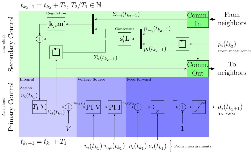
Figure 5: Distributed primary and secondary control strategy implemented at the i-th converter.
vectors concatenating the local value and the incoming signals. Note that the delay blocks are introduced in order to "wait" for the communication from the other nodes. The secondary level consist on a consensus power sharing controller with an auxiliary mean voltage regulation loop, in such a way that the voltage reference for they primary level does not deviate much from the nominal value, while the injected power by all sources is done proportionally.
We assume that the different units have independent clocks, but they are accurate enough to enforce actuation at exactly the same rate , . We can state a counter, on the discrete actuation instants at the primary level so that . Because the secondary level dynamics are much slower than at the primary level, we can also assume that actuation is perform at a slower rate and that . We can also state a counter, on the discrete actuation instants at the secondary level so that .
3.2. Primary Control
3.2.1 Average Measurements
In order to obtain voltage, current, and power signals for feedback, the measurement device can be considered a low pass filter with the simple transfer function
where is the signal to be measured (at each node: battery voltage , capacitor voltage , inductor current , and output power ) and its measurement after the filter. The cut-off frequency of the filter is given by which can be chosen arbitrarily. The behavior of this filter at the simulation rate given by T > 0 can be approximated by the following differences equation
3.2.2 Feed-Forward
Following the standard argument on the mean charge and discharge times of each inductor, when , we have that the static behavior between the voltages and the duty cycle at each boost satisfy
Solving for the duty cycle leads to propose a controller that feed-forwards the battery voltage:
As the battery voltage cannot be directly manipulated, it represents a perturbation, and so this strategy can help to avoid undesired dynamics from malfunctioning batteries and it also linearizes the steady state behavior of the system.
A saturation over the value of the duty cycle can also be considered:
with and arbitrary saturation values.
Note the intrinsic delay of the implementation of the primary controller. To assure that actuation is perform at a regular rate, the controller enforces its output at the beginning of each interval, relaying on the possible time varying computation performed in the previous interval. In this way, independently of the time needed to compute the values, the actuation over the plant is carried on at a regular basis.
As with the voltage in (8), the static relationship for the current corresponds to
Evaluating this and (8) at and replacing the feed-forward expression (9) leads to:
with approximations that hold when the perturbation signals and are constant, and constant. Because the switching process is faster than the primary controller, these equations represent an average discrete time model of the boost converter described by a states matrix with eigenvalues and . To stabilize this system, a control law that feedbacks both states can be proposed as in the following subsection.
3.2.3 Voltage Source Implementation
The input of the feed-forward part of the controller is obtained from a control loop whose objective is to implement a voltage source with unit gain. This is typically done through a current and voltage feedback in cascade (See for example ). The current controller can be implemented as a discrete PI controller with the following equations:
Where the constants
are given in terms of the proportional constant and the integral time .
The current reference, , for this loop comes from a voltage PI controller implemented by the following equations:
with constants
depending on the proportional constant and the integral time .
In this way, both states and are used for feedback and so it is possible to achieve a unitary steady state gain between the voltage reference and the node voltage measurement when the controller parameters are adequately chosen.
3.2.4 Integral Action
If the input of the voltage PI controller changes at a slow rate and within a relatively small region around the nominal value, then the boost converter can behave close to an ideal voltage source when all the control parameters are well tuned. To achieve this behavior of the reference, an integral action over the voltage deviation can be implemented with the following equations:
In this way, the primary control input is the signal , which represents the desired change rate of the node voltage deviation from the nominal value V > 0; and represents intern states of the primary layer.
The input to the primary level controller is determined by the secondary level at a slower rate. If a primary action instant coincides with a secondary one, that is, if , and the speed rate between both clocks is given by , then there are n primary steps in every secondary step and so the previous secondary action instant coincides with the n-th previous primary instant: .
From (12), we can write,
when the input is constant . That is, the integral action at the primary level can also be seen as an integral action at the secondary rate.
3.3 Secondary Control
3.3.1 Secondary Level Objectives
One common secondary level control objective is Power Sharing, or the ability of the controlled voltage sources to inject or absorb power in a predefined proportion. That is, ,
with a known per unification constant. The last expression defines a consensus problem and it is typically addressed with a power feedback.
As power sharing is a consensus problem, equation (13) can be written in terms of convergence to the origin of an error vector like in [31]. Consider a transformation defined from an incidence matrix of a directed tree to define an error vector
where are the injected powers in per-unit, and matrix is the pseudo-inverse of , such that and . It can be shown that equation (13) is equivalent to 0.
As a result of the power sharing control strategy, the voltages at each node deviate from their nominal value, and therefore an additional objective for the entire micro-grid is voltage regulation. A linear definition of this can be stated as
where the elements of add up to one ( ) in such a way that represents a weighted average of the nodes voltages. Particular interesting cases are to obtain average voltage regulation, and to force the i-th node to operate at nominal voltage.
We can define the per unit voltage deviation, , in such a way that . In vector form, . If the average voltage deviation approximates the origin, then we have that
and voltage regulation is achieved.
3.3.2 Communication Dynamics
In order to implement any distributed secondary strategy, communication between the different agents is needed. In a realistic scenario, the model of this process needs to consider delays and information lost. Furthermore, the communication link between each node can present different dynamic and stochastic behavior. These problems can be diminish if the actuation rate of the secondary controller is slower than the expected communication time, in order to "wait" for the correct information to arrive from the neighbors. In this way, the communication process can be considered as a delay of the secondary clock.
To simulate the communication process from the j-th to the i-th agent, we consider a function of time in such a way that,
That is, the per unit power and the voltage deviation reference at the primary level of the j-th node, available for the i-th node at instant t. We consider these two variables because they will be used for the secondary level feedback in order to achieve the stated control objectives. We will consider that the communication from j to i success with a known fixed probability .
With this, we can model de communication process of the entire microgrid with help of matrices and in such a way that their elements are given by
Note that the previous matrices consider all possible communication channels and the N own feedback signals from each agent, independently of which channels are actually considered by the control strategy. That is, the communication problem ("how should information be shared?") is considered independent of the control problem ("which information should be shared?"). Furthermore, the communication problem is treated independently for each ordered pair of nodes, not assuming any correlation between channels.
In the ideal case with lossless communication, all columns of the communication matrices are equal so and with .
3.3.3 Distributed Control Strategy
Adopting the notation introduced in the previous discussion, at each node , the secondary control action can be computed at every instant according to the following discrete time control law
The feedback matrix is chosen to achieve Power Sharing similar as the strategies reviewed in, e.g., [23–26, 32]. Although we consider that it is obtained as the negative Laplacian matrix of the weighted undirected graph , it is also possible to use other
matrices with the zero sum row property, L1 = 0. In any case, communication will be needed in every case where the off-diagonal elements of L are non-zero.
The vector , , is considered in order to achieve voltage regulation through a feedback of the voltage deviation reference, i.e. of the integration action at the primary level. Note that if and for some K > 0, then there is no need of communication to implement this part of the controller. As far as the authors know, this auxiliary loop has not been proposed for DC systems in other references with similar power sharing mechanisms.
With lossless communications, equation (17) can be stated for all nodes as
3.3.4 Convergence Criteria At Secondary Level
To corroborate that the discrete time implementation of the secondary level controller stabilizes the closed loop system, the following theorem gives sufficient convergence conditions for power sharing and voltage regulation under ideal conditions.
Theorem 1 (Power sharing and voltage regulation). With lossless communication, ideal voltage sources, and L1 = 0, if Power Sharing and Voltage Regulation are achieved when the load of the system is constant then the eigenvalues of matrix
are smaller in module than one (are within the unit circle).
Proof. If primary level controllers are properly tuned, the sources resemble ideal ones and so:
In terms of the voltage deviation , the last equation can be expressed as
From the secondary level perspective, as the sources are assumed close to ideal, the dynamic behavior of the entire system is dictated by the integral actions in equation (12). Combining with (18) we obtain:
On the other side, rearranging the voltage deviation vector as a diagonal matrix in such a way that , the per unit power injected by all the boost sources in equation (4) can be written in vectorial form as
where is a per-unification matrix and the vectors and correspond respectively to the injected power by the voltage sources and the consumed power by the perturbations in per-unit.
If the voltage deviations are small(if ), it makes sense to approximate the previous quadratic expression(20)by a Taylor linearization(see [26])given by:
When the communication process introduces a unit delay but does not present information losses, the secondary level control strategy (17) can be written in terms of the consensus error and the average deviation:
when L1 = 0. Using this, (19), and (21), we can write for the consensus error :
and for the average voltage deviation:
Therefore, the entire linearized system can be written as:
with as defined before and .
From Lyapunov's first method, if the eigenvalues of are within the unit circle, then the solution of the non-linear system at the secondary level converges. Therefore, a necessary (but not sufficient) condition for power sharing and voltage regulation with constant load (i.e. with ), is that matrix is Schur (has all its eigenvalues within the unit circle).
Remark 1. Naturally, the eigenvalues of can be used to describe the dynamic behavior of and . For the influence of the per unit load change, , over the consensus error, e, robust control arguments can be used in the vicinity of the operation point. In particular, from equation (22), the -norm of the transfer function matrix between the load change rate and the error can be interpreted as a measurement of Power Sharing Accuracy because when is Schur.
Remark 2. Additionally, in a similar way as in [26], the non-linear equation (20) can be used to study less restrictive convergence criteria in terms of operation regions of the voltage deviations. In this way, robustness of the closed loop system against voltage changes can be characterized numerically.
Remark 3. In this way, the previous result allows to easily check for power sharing and voltage regulation, and to compare the performance of different controllers through numeric indicators. This observations can be further developed to define control design procedures. Note that when , or when , matrix becomes block-triangular and its eigenvalues are dictated by the diagonal blocks.
IV. TRAJECTORY COMPUTATION
4.1 Software Implementation
Because the differential equations of the closed loop model are explicitly solved, dynamic trajectory computation of the described set-up can be efficiently implemented in any language. To do so, a basic algorithm is detailed as follow. At each instant, :
1.- Choose pre-calculated matrices and according to the current switching configuration.
2.- Update states using equation (6).
3.- For each node :
i) Update measurements using filters (7).
ii) If it is a secondary control instant:
-
Read communicated signals.
-
Update primary level input according to equation (17).
iii) If it is a primary control instant:
-
Integral action in equation (12).
-
Voltage PI in equation (11).
-
Current PI in equation (10).
-
Feed forward in equation (9).
iv) Update switching position by PWM.
j) If it is a secondary control instant:
- Update communicated signals in equations (15) and (16).
In order to obtain faster performances, the previous basic procedure can be modified to exploit specific characteristic of the chosen language, e.g. vectorization instead of looping; or saving variables at a slower rate. Furthermore, if then every secondary control instant is also a primary control instant, and so this decision does not need to be checked at every simulation instant. Further improvements can also be proposed and evaluated in any specific hardware/software configuration. However, there is no need of using specialized or tailor made solutions.
Table 1: Boost Sources Parameters
| i | 1 | 2 | 3 | 4 | 5 |
| $L_i[mH]$ | 0.7417 | 0.7437 | 0.7457 | 0.7458 | 0.7513 |
| $C_i[mF]$ | 4.4911 | 4.5264 | 4.4617 | 4.5360 | 4.4321 |
| $K_{P,I,i}$ | 1.5 | ||||
| $T_{I,I,i}$ | 0.01 | ||||
| $K_{P,V,i}$ | 2.4 | ||||
| $T_{I,V,i}$ | 0.01 | ||||
| $d_{min}$ | 0.2 | ||||
| $d_{max}$ | 0.8 |
4.2 Example Micro-Grid Description
Consider the micro-grid in Figure 2 with N = 5 active nodes and a nominal voltage V = 24[V]. At each node, a boost converter is connected with nominal battery voltage E = 12[V]. For all nodes, the PWM process is carried out at a frequency of . The individual parameters of these sources are given in Table 1. All nodes are designed to inject nominal power and all measurement filters have the same time constant .
The graph that describes the edges of the micro-grid is given in Figure 6. The resistances associated to each edge can be seen in Table 2. For all the simulations, we assume that the perturbations (battery voltage and load power) behave as in Figure 7. Note that the loads present abrupt step changes and continuously varying changes.
4.3 Primary Control Simulation
The primary control layer is implemented locally at each node, however and for simplicity, the current and voltage PI parameters are the same for every machine. These values can also be seen in Table 1. We assume that the primary actuation is performed at a rate of , while the simulation step is .
Figure 6: Micro-grid graph C and consensus directed tree for numeric examples
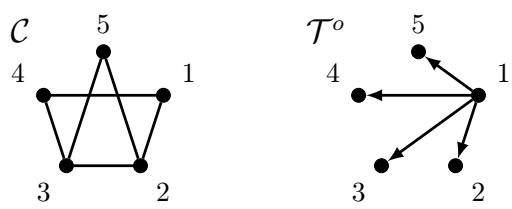
Table 2: Grid Lines Parameters. i j
| i | j | $R_{ij}[\Omega]$ |
| 1 | 2 | 0.5044 |
| 1 | 4 | 0.4988 |
| 2 | 3 | 0.5008 |
| 3 | 4 | 0.4902 |
| 3 | 5 | 0.4936 |
| 2 | 5 | 0.5059 |
Figure 8 shows the behavior of the micro-grid with only the primary control layer. That is, the secondary loop action is ignored so that the voltage reference at the primary level are forced to be equal to the nominal value: . Although the signals present significant ripple because of the switching process, it is clear that the voltages remain around the nominal value. Because of the feed-forward strategy, changes in the battery voltage disturb the voltage only during a brief transient. As there is no power feedback considered, the injected power by each node follows the changes of the load demand. However, the voltage is always restored to the nominal value, thus showing that the primary level implementation of the voltage sources is successful.
4.4 Secondary Control Simulation
Consider a power sharing secondary controller described by a Laplacian matrix derived from the micro-grid graph C in the following way:
That is, each node needs to share information only with its physical neighbors. For each edge and in both directions, we will consider that a communication link has a success probability of , . Lower success probabilities could also be considered without affecting much the overall performance. The secondary clock is given by .
With a matrix k = 0, the behavior of the micro-grid with the specified disturbances can be seen in Figure 9. Note how power sharing is achieved within the ripple space and all the sources modify their voltages to inject power proportional to the total load. However, the voltages mean value deviates systematically from the nominal value.
{"image_source":{"path":"images/0d8ca786c210eaac333981aa4858021c2cebe39a4e64b2290ffa1a060b94e5ad.jpg"},"content":"","chart_caption":[],"chart_footnote":[]}
{"image_source":{"path":"images/1ff594cf4d0b73f2c31cab941c17e67d82dfb221fc588c2577233eda514723e6.jpg"},"content":"","chart_caption":[],"chart_footnote":[]}
{"image_source":{"path":"images/d20aec95fe1deaffbc2899a3c9b5940846dc99d5b201f7dd012b1be1f6842e3b.jpg"},"content":"","chart_caption":[{"type":"text","content":"Figure 7: Perturbations for the example micro-grid. a) Battery voltage in [p.u.], and b) Load power consumption in [p.u.]"}],"chart_footnote":[]}
{"image_source":{"path":"images/68ea61bff08c0f7edd28111b42ada97e00e1aa74a15ec9e4433dbea401210050.jpg"},"content":"","chart_caption":[{"type":"text","content":"Figure 8: Behavior of micro-grid with only primary control. a) Node voltages in [p.u.], and b) Injected power in [p.u.]"}],"chart_footnote":[]}
To improve average voltage regulation around the nominal value, i.e. with , consider the matrix
Note that to implement this part of the controller all communication channels are needed. In this case, Figure 10 shows the behavior of the microgrid. Power sharing is still achieved, but the voltages are such that their average value always is approximately the nominal value. Consequently, considering the directed tree in Figure 6, and the consensus transformation , the eigenvalues of matrix are all contained in the unit circle satisfying the convergence criteria. In the case where , the eigenvalue associated to the mean voltage deviation is identically one, and therefore this quantity cannot converge to the origin as confirmed by the simulation in Figure 9.
4.5. Comments on Simulation Speed
All previous simulations were obtained with a time step . In all cases the ratio between computation and simulation time is around .
{"image_source":{"path":"images/ec904b00f005567834643fab044b5d8cb00c452a709ca1f8cc9955d86d88b3b2.jpg"},"content":"","chart_caption":[],"chart_footnote":[]}
{"image_source":{"path":"images/3c569ce6e031aabb552303f23eb447e91620be2ba0138640c4526dd5c29d45e3.jpg"},"content":"","chart_caption":[],"chart_footnote":[]}
{"image_source":{"path":"images/11d4ecbe6e0bedf1725a518a1839fdf75a1a7c5d4f0b3e2d0a2124f49dfd5e51.jpg"},"content":"","chart_caption":[{"type":"text","content":"Figure 9: Behavior of micro-grid with power sharing control. a) Node voltages in [p.u.], and b) Injected power in [p.u.]"}],"chart_footnote":[]}
{"image_source":{"path":"images/a810c5e8d5ecf59a33d4d2c8e50fac3065592c46f496b98500d37bbb8a8be9e2.jpg"},"content":"","chart_caption":[{"type":"text","content":"Figure 10: Behavior of micro-grid with full secondary control. a) Node voltages in [p.u.], and b) Injected power in [p.u.]"}],"chart_footnote":[]}
That is, to obtain the 10[s] shown in the graphs, around 80[s] were needed. Naturally, the simulation time depends on the time step used and faster simulations can be obtained by modifying this parameter. For example, Figure 11 shows the same micro-grid simulated with and a resulting computation ratio . This is done in a standard notebook, without any dedicated hardware or software implementation.
As is also clear from Figure 11, the speed gained by decrementing the simulation time step implies less precision. On the contrary, with , and a resulting ratio of , Figure 12 shows the evolution of the system with much less numeric noise.
V. CONCLUSION
This paper focuses on DC micro-grids in mesh topology, where each node is actuated through a voltage source implemented by a storage device and a boost converter, and with loads or distributed generation units as arbitrary perturbations. We propose a general algorithm to compute the states trajectory of the closed-loop system, which considers switching devices, their hardware interconnections, a two-level control hierarchy with different actuation rates, measurement and communication dynamics, and can be used for aiding implementation of hardware-in-the-loop or real-time simulations, as well as for convergence analysis.
{"image_source":{"path":"images/5dfaf915e5792a2f538d19e5d2838b984579c5666c73e494be98e386a303e131.jpg"},"content":"","chart_caption":[],"chart_footnote":[]}
{"image_source":{"path":"images/873861cc9715e4d6c085c44cef52f190002502f37179fec08aaf83601539ee43.jpg"},"content":"","chart_caption":[],"chart_footnote":[]}
{"image_source":{"path":"images/3ef7430c885839a0c72c33e020eba9495205850e8203527794b0b8ddc34b2c0f.jpg"},"content":"","chart_caption":[],"chart_footnote":[]}
{"image_source":{"path":"images/08dbfa3b02bb49845a51aa82baf6f147c0bc6c84b551647f9ecfac1d5a581689.jpg"},"content":"","chart_caption":[{"type":"text","content":"Figure 11: Behavior of micro-grid with full secondary control and "},{"type":"equation_inline","content":"\overline{T}"},{"type":"equation_inline","content":"10[\mu s]"},{"type":"text","content":" . a) Node voltages in [p.u.], and b) Injected power in [p].u."},{"type":"text","content":"Figure 12: Behavior of micro-grid with full secondary control and "},{"type":"equation_inline","content":"T = \overline{0}.5[\mu s]"},{"type":"text","content":". a) Node voltages in [p.u.], and b) Injected power in [p.u.]"}],"chart_footnote":[]}
Our primary level control includes filtered measurements, a non-linear feed-forward strategy, current and voltage PI-loops, and an integral action to actuate the switching devices as voltage sources. We present necessary conditions for convergence of the secondary level closed-loop system, which considers a consensus algorithm to achieve power sharing and a novel additional loop to reach average voltage regulation.
In contrast to idealized continuous-time dynamics, our explicit discrete-time modeling brings the convergence analysis closer to its final hardware implementation, allowing for more accurate simulation mechanisms and stability criteria. Overall, our approach provides a comprehensive solution for DC micro-grid control in mesh topology, considering the complex dynamics involved and their practical implementation.
Conflict of Interest
The authors declare no conflict of interest.
Ethical Approval
Not applicable
Data Availability
The datasets used in this study are openly available at [repository link] and the source code is available on GitHub at [GitHub link].
Funding
This work did not receive any external funding.
References
Cite this article
Related Research



Special Issue
Launch a focused special issue to highlight research, emerging trends, and expert insights in your academic field.
