




IntelliPaper
Abstract
This document shows the required format and appearance of a manuscript prepared for SPIE journals.
It is prepared using LaTeX2e with the class file spieman.cls. Please note that the following journals require the use of structured abstracts in manuscript submissions: Neurophotonics, the Journal of Biomedical Optics, and the Journal of Medical Imaging. Structured abstracts are encouraged for the Journal of Micro/Nanolithography, MEMS, and MOEMS. Guidelines are available on the journal website. Whether structured or single-paragraph, the abstract should be a summary of the paper and not an introduction. Because the abstract may be used in abstracting and indexing databases, it should be self-contained (i.e., no numerical references) and substantive in nature, presenting concisely the objectives, methodology used, results obtained, and their significance. A list of up to six keywords should immediately follow.
Explore Digital Article Text
I. INTRODUCTION
Attention mechanisms have become a fundamental component of deep learning models, including the field of computer vision, where spatial understanding plays a crucial role. A wide range of attention mechanisms have been designed to enable models to focus on the most relevant parts of input images, leading to improved performance and enhanced interpretability of the models' decision-making processes.
The origins of attention in deep learning can be traced back to the revolutionary works in natural language processing (NLP), introduced as a way to address the limitations of traditional sequence-to-sequence models, such as the inability to effectively capture long-range dependencies. The initial success of attention mechanisms in NLP tasks, such as machine translation and language modeling, inspired researchers to explore their potential in other domains, including computer vision.
In the computer vision domain, attention mechanisms have been adapted to various tasks, such as image classification, object detection, and semantic segmentation. The key idea behind these attention mechanisms is to allow the model to dynamically focus on the most relevant spatial regions of the input image, rather than treating all regions equally. The selective focus has been shown to improve the model's performance and provide better interpretability of its decision-making.
However, the traditional approaches to attention mechanisms in computer vision often suffer from a lack of smoothness in the attention maps, resulting in sharp transitions that negatively affect model generalization. This problem of spatial incoherence is particularly pronounced in the task of semantic segmentation, where accurate pixel-level predictions require a detailed understanding of the spatial relationships within the image.
Semantic segmentation, the task of assigning a semantic label to each pixel in an image, relies heavily on capturing fine-grained details and understanding the spatial context. The existing attention mechanisms struggle to effectively capture the detailed relationships within the image due to the abrupt pixel-level transitions in the attention maps. This inconsistency in the attention maps often leads to inaccurate segmentation boundary predictions and a tendency for the model to overfit on the training data, limiting its ability to generalize well on unseen images.
Additionally, the lack of smoothness in attention maps can make models susceptible to noise. Small perturbations in the input image may drastically alter the attention weights, causing unstable predictions. Such sensitivity to noise is particularly problematic in real-world scenarios where images are often corrupted by artifacts or imperfections.
To address these limitations, we present a new approach called Smooth Attention that incorporates a smoothness constraint, encouraging gradual changes in attention weights and mitigating the risks of sharp transitions or noise sensitivity. By enabling a detailed understanding of spatial relationships within the image, Smooth Attention leads to higher-level performance on tasks where spatial coherence is crucial, such as image semantic segmentation.
1.1 Related Work
The Smooth Attention methodology builds on the successful implementation of attention mechanisms in computer vision, particularly within transformer-based architectures such as the Vision Transformer and Swin Transformer. Our primary focus is the enhancement of the spatial coherence within a single attention layer, drawing inspiration from attention integration techniques in convolutional neural networks (CNNs), including Non-local Neural Networks and the Convolutional Block Attention Module (CBAM).
Spatial coherence has been a focal point in various applications, including image segmentation with CRF-RNN and image generation through PatchGAN. Smooth Attention introduces adaptive computation elements akin to Adaptive Computation Time for recurrent neural networks (RNNs), selectively applying smoothing techniques.
Our framework is inspired by recent innovations in Attention Augmented Convolutional Net- works and Focal Self-attention. By leveraging the Chebyshev distance, we align with the principle of dynamically adjusting kernel weights based on local features during convolutional operations.
The spatial coherence component of our approach resonates with the foundational concepts of CoordConv, as it explicitly encodes spatial information into convolutional layers. Moreover, our methodology exhibits parallels with the Performer architecture, which reduces computational complexity while maintaining high performance by approximating attention through random feature maps.
Building on the principles of adaptive filtering as outlined in by Solomon et al., we effectively combine original and smoothed attention scores based on identified variations. Such selective smoothing enhances the established concept of gating in GRCNN, enabling precise control over the influence of neighboring attention scores and pixels while preserving critical features.
II. METHODOLOGY
In this section, we present a new attention mechanism in convolutional neural networks called Smooth Attention. The module is designed to enhance the spatial coherence of attention maps while maintaining the flexibility and power of traditional attention mechanisms. Our approach addresses the issue of inconsistent or "noisy" attention patterns that oftentimes arise in standard attention mechanisms, particularly in vision tasks where spatial coherence is crucial, like image segmentation of complex-shaped objects.
2.2 Architecture Overview
The Smooth Attention approach is implemented as a neural network module. It consists of three main components:
1. Query, key, and value projections (3.1.1)
2. Attention computation (3.1.2)
3. Smoothness enforcement mechanism (3.1.3)
Each of these components plays a crucial role in achieving the final goal of spatially coherent attention.
3.3 Query, Key, and Value Projections
The first step in the Smooth Attention module is the projection of the input tensor X into query (Q), key (K), and value (V) spaces. The projection is achieved using 1x1 convolutions (1), (2), (3).
Where [Conv1x1] represents a convolutional layer with a 1x1 kernel. The final projections serve multiple purposes:
-
Allow the network to learn representations of the input that are suitable for computing attention.
-
Enable the module to adjust the channel dimensionality, reducing computational complexity.
-
Provide a learned transformation that emphasizes or suppresses aspects of the input for attention computation.
2.4 Attention Computation
After obtaining the projected tensors, we compute the attention scores using the scaled dot-product attention mechanism, similar to the one used in Transformer architectures, shown in (4):
Where:
4. represents the matrix multiplication of Q and the transpose of K;
5. is the dimensionality of the key vectors;
-
is used for scaling to counteract the effect of large dot products in high dimensions;
-
Softmax is applied to normalize the attention scores.
The computation results in the attention map where each position attends to all other positions, capturing global dependencies in the input.
2.1.3 Smoothness Enforcement Mechanism
The key concept in the Smooth Attention module is the introduction of a smoothness enforcement mechanism. The mechanism is designed to address the spatial incoherence in vision attention when nearby pixels may have radically different attention weights.
To enforce the smoothness, we_compute the Chebyshev distance between each pixel's attention distribution and those of its eight neighboring pixels. The Chebyshev distance is defined as the maximum absolute difference across all dimensions (5).
We compute this distance for each of the eight neighbors and take the maximum:
The choice of Chebyshev distance over other metrics is motivated by its sensitivity to the largest difference in any single dimension, which aligns well with the goal of detecting abrupt changes in attention patterns.
2.2 Smoothness Thresholding and Mask Creation
If the maximum Chebyshev distance exceeds a predefined threshold (a value between 0 and 1), we consider the attention at that pixel to be non-smooth. We create a binary mask where 1 indicates non-smooth regions and 0 indicates smooth regions (7).
2.3 Attention Application with Smoothness Consideration
The smoothing mask is then used to selectively apply the attention mechanism. In smooth regions, we allow the full attention mechanism to operate, while in non-smooth-regions, we reduce the influence of the attention mechanism:
Where:
-
γ is a learnable parameter initialized to zero;
-
V is the value projection of the input;
-
x is the original input.
The learnable parameter allows the network to gradually incorporate the attention mechanism as training progresses. A soft start is used to help stabilize the training process and allow the network to learn "when and how much" to rely on the attention mechanism.
Due to its structure, Smooth Attention module offers several advantages:
-
Spatial Coherence: By enforcing local smoothness, the module encourages the production of more coherent attention maps, improving model's performance on complex computer vision tasks.
-
Noise Reduction: The smoothness constraint acts as a form of regularization, reducing the impact of noise and spurious correlations in the attention computation.
-
Interpretability: Smoother attention maps are more interpretable, providing clearer insights into which parts of the input the model is focusing on.
-
Adaptive Mechanism: The learnable parameter and the smoothness threshold provide additional level of engineering flexibility, allowing the network to adapt the strength of the smoothness constraint based on the task and data.
The Smooth Attention module extends traditional attention mechanisms by incorporating a local smoothness constraint. The constraint is enforced through applying the Chebyshev distances in the attention space, resulting in more coherent and accurate attention maps for convolutional neural networks. The module's design allows for a flexible trade-off between global attention capabilities and local coherence, making it adaptable to a wide range of vision tasks dependent on the spatial coherence level.
III. EXPERIMENTS
To demonstrate the effectiveness of Smooth Attention, we perform experiments on five diversified image segmentation datasets, including the Caltech-UCSD Birds-200-2011, Large-Scale Dataset for Segmentation and Classification, Fire Segmentation Image Dataset, Kvasir-Instrument: Diagnostic and Therapeutic Tool Segmentation Dataset in Gastrointestinal Endoscopy, and Flood Semantic Segmentation Dataset.
To explore the influence of the attention module, we implement a custom model with the U-Net architecture which is a popular choice for semantic segmentation tasks. We use ResNet18 as the encoder, which is followed by the Smooth Attention mechanism to help the model focus on important features. The decoder is implemented as a series of transposed convolutions that upscale the feature map. Each transposed convolution is followed by a ReLU activation, except for the last one. The decoder gradually increases the spatial dimensions while reducing the number of channels. The final layer outputs the same number of channels as the number of classes for segmentation. The complete model architecture is demonstrated in Figure 1.
We perform experiments across multiple smoothness thresholds (from 0.1 to 0.9 with a 0.1 step) for each dataset, and compare the results with a threshold of 2.0 that illustrates the model without attention mechanism in place (any value above 1.0 means no smoothing constraint applied). All datasets are split into 80% for training, and 20% for testing. We choose IoU, Dice Coefficient, Test Accuracy, Test Precision Test F1 Score as metrics to compare the final results.
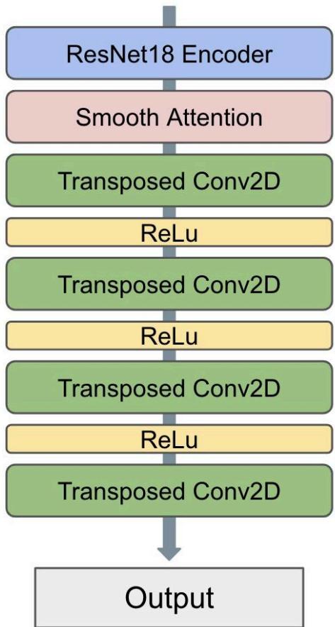 Fig. 1: Model Architecture
Table 1: Experiments for Caltech-UCSD Birds-200-2011 results
| Metric | Test IOU | Test Dice | Test Acc | Test Prec | Test Recall | Test F1 |
| 0.1 | 0.7933 | 0.9231 | 0.9686 | 0.7674 | 0.9838 | 0.8550 |
| 0.2 | 0.8028 | 0.9294 | 0.9670 | 0.7457 | 0.9829 | 0.8430 |
| 0.3 | 0.7997 | 0.9292 | 0.9672 | 0.7641 | 0.9829 | 0.8521 |
| 0.4 | 0.7894 | 0.9186 | 0.9679 | 0.7654 | 0.9799 | 0.8495 |
| 0.5 | 0.7963 | 0.9258 | 0.9672 | 0.7609 | 0.9827 | 0.8494 |
| 0.6 | 0.7949 | 0.9260 | 0.9693 | 0.7740 | 0.9812 | 0.8562 |
| 0.7 | 0.7952 | 0.9239 | 0.9677 | 0.7685 | 0.9811 | 0.8526 |
| 0.8 | 0.8003 | 0.9272 | 0.9678 | 0.7700 | 0.9808 | 0.8493 |
| 0.9 | 0.7994 | 0.9229 | 0.9699 | 0.7881 | 0.9823 | 0.8610 |
| 2.0 | 0.7909 | 0.9222 | 0.9667 | 0.7497 | 0.9827 | 0.8453 |
The results for Caltech-UCSD Birds-200-2011 can be observed in Table 1. The superior performance of the Smooth Attention mechanism at lower smoothness thresholds (0.1, 0.2, 0.3) compared to the model without attention (threshold of 2.0) suggests that the attention module is effectively helping the model in focusing on the most relevant features in the image segmentation task. By applying the smoothness constraint, the attention mechanism is able to selectively high-light most informative regions of the input, leading to better segmentation accuracy, IoU, and Dice coefficient metrics.
We see the consistently high Test Recall values across all smoothness thresholds, showing that the model is able to correctly identify most of the positive instances in the test set, regardless of the attention mechanism's configuration. Similar to IoU, the Dice coefficient peaks at a lower smoothness threshold, demonstrating that low levels of attention smoothness provide better balance between focus and flexibility in feature selection. At the same time, the highest accuracy and pre-cision occur at a higher threshold, suggesting that for overall pixel-wise classification a smoother attention map reduces the noise and the number of false positives. The recall peak occurs at the lowest smoothness threshold, since true positives can be captured at a strict threshold easier. By applying a stricter smoothness constraint, the attention module is able to capture important visual cues, maximizing the model's ability to detect positive instances in the data.
The experiment results for the Large-Scale Dataset for Segmentation and Classification can be observed in Table 2. The stronger IoU and Dice coefficient performance at lower smoothing thresholds indicates that the model is more effective in identifying variances in the input image data at strict thresholds. Such behavior unveils the rich tapestry of diversity within the fish segmentation data, highlighting the necessity for fine-grained approaches to capture the complexities of the images.
Table 2: Large-Scale Dataset for Segmentation and Classification.
| Metric | Test IOU | Test Dice | Test Acc | Test Prec | Test Recall | Test F1 |
| 0.1 | 0.9344 | 0.9764 | 0.9882 | 0.9426 | 0.9904 | 0.9618 |
| 0.2 | 0.9364 | 0.9784 | 0.9887 | 0.9434 | 0.9916 | 0.9638 |
| 0.3 | 0.9309 | 0.9749 | 0.9879 | 0.9493 | 0.9901 | 0.9600 |
| 0.4 | 0.9320 | 0.9751 | 0.9883 | 0.9399 | 0.9898 | 0.9627 |
| 0.5 | 0.9355 | 0.9787 | 0.9886 | 0.9426 | 0.9910 | 0.9630 |
| 0.6 | 0.9283 | 0.9706 | 0.9874 | 0.9383 | 0.9872 | 0.9602 |
| 0.7 | 0.9247 | 0.9694 | 0.9886 | 0.9519 | 0.9866 | 0.9620 |
| 0.8 | 0.9290 | 0.9731 | 0.9885 | 0.9434 | 0.9882 | 0.9626 |
| 0.9 | 0.9336 | 0.9759 | 0.9879 | 0.9465 | 0.9899 | 0.9612 |
| 2.0 | 0.9363 | 0.9781 | 0.9886 | 0.9436 | 0.9915 | 0.9611 |
Consistently high accuracy scores for all thresholds, including 2.0 (no attention), showcase the absence of background complexity within image data, helping the model be accurate in object segmentation with and without smoothing. Still, slight improvements can be seen when attention smoothing is applied with peak scores seen at thresholds of 0.2, 0.5 and 0.7.
Precision metric demonstrates the best result at a threshold of 0.7, showing accurate prediction of pixel-level distribution. The higher thresholds can be more beneficial for tasks requiring broader feature recognition helped by greater noise suppression and lesser sensitivity to variation in input data. Moreover, high values of Recall and F1 Score at lower thresholds are a clear representation of the model's effectiveness in capturing critical details due to strict smoothing masks.
Table 3 demonstrates the results for the Fire Segmentation Image Dataset. The IoU and Dice coefficient peaked at a smoothing threshold of 0.4, with strong performance also observed at 0.5 and 0.6. This behavior can be attributed to the special characteristics of fire images in the dataset.
Table 3: Fire Segmentation Image Dataset Fire scenes typically exhibit complex, irregular shapes with varying intensity and color gradients, making them challenging to segment accurately.
| Metric | Test IOU | Test Dice | Test Acc | Test Prec | Test Recall | Test F1 |
| 0.1 | 0.8484 | 0.9228 | 0.9904 | 0.4903 | 0.9630 | 0.6322 |
| 0.2 | 0.8512 | 0.9246 | 0.9913 | 0.4868 | 0.9633 | 0.6403 |
| 0.3 | 0.8488 | 0.9189 | 0.9925 | 0.5269 | 0.9599 | 0.6377 |
| 0.4 | 0.8518 | 0.9277 | 0.9914 | 0.4907 | 0.9662 | 0.6446 |
| 0.5 | 0.8501 | 0.9248 | 0.9910 | 0.4753 | 0.9648 | 0.6329 |
| 0.6 | 0.8507 | 0.9268 | 0.9919 | 0.5096 | 0.9656 | 0.6489 |
| 0.7 | 0.8498 | 0.9231 | 0.9918 | 0.5027 | 0.9628 | 0.6460 |
| 0.8 | 0.8480 | 0.9208 | 0.9918 | 0.5057 | 0.9594 | 0.6520 |
| 0.9 | 0.8497 | 0.9231 | 0.9915 | 0.4888 | 0.9608 | 0.6314 |
| 2.0 | 0.8504 | 0.9211 | 0.9911 | 0.4837 | 0.9623 | 0.6399 |
The dataset's nature, featuring dynamic fire boundaries and potential smoke interference, explains why moderate smoothing thresholds (0.4 - 0.6) outperform others. At these levels, the algorithm effectively balances detail preservation and noise reduction. Lower thresholds (0.1 - 0.3) likely retain too much noise and small, irrelevant features, while higher thresholds (0.7 - 0.9) risk oversimplifying the fire's complex structure.
Consistently high values of Accuracy and Recall suggest the model's ability to correctly identify true positives and relevant instances in the image dataset, regardless of whether smoothing is applied. However, attention smoothing does lead to marginally improved performances in these metrics.
The balanced approach to smoothing not only improves traditional segmentation metrics like IoU and Dice coefficient but also enhances the model's overall predictive capabilities across a broader range of performance indicators.
Table 4: Kvasir-Instrument: Diagnostic and Therapeutic Tool Segmentation Dataset in Gastrointestinal Endoscopy
| Metric | Test IOU | Test Dice | Test Acc | Test Prec | Test Recall | Test F1 |
| 0.1 | 0.9105 | 0.9405 | 0.9853 | 0.9427 | 0.9370 | 0.9138 |
| 0.2 | 0.9248 | 0.9536 | 0.9881 | 0.9489 | 0.9674 | 0.9294 |
| 0.3 | 0.9223 | 0.9504 | 0.9876 | 0.9632 | 0.9548 | 0.9263 |
| 0.4 | 0.9071 | 0.9348 | 0.9852 | 0.9231 | 0.9367 | 0.9136 |
| 0.5 | 0.9125 | 0.9420 | 0.9848 | 0.9162 | 0.9364 | 0.9163 |
| 0.6 | 0.9054 | 0.9371 | 0.9847 | 0.9077 | 0.9326 | 0.9167 |
| 0.7 | 0.9052 | 0.9374 | 0.9828 | 0.9121 | 0.9345 | 0.9081 |
| 0.8 | 0.9093 | 0.9394 | 0.9861 | 0.9083 | 0.9587 | 0.9217 |
| 0.9 | 0.9091 | 0.9390 | 0.9857 | 0.9115 | 0.9470 | 0.9197 |
| 2.0 | 0.9108 | 0.9376 | 0.9855 | 0.9152 | 0.9479 | 0.9208 |
Table 4 presents the results of the Kvasir-Instrument: Diagnostic and Therapeutic Tool Seg- mentation Dataset in Gastrointestinal Endoscopy. The dataset contains images of the commonly used gastrointestinal endoscopy surgical tools that pose challenges for segmentation models due to the shape complexity of the surgical tools captured in the scenes.
The best performance across numerous evaluation metric criteria can be seen at lower thresholds (0.1-0.3) with peak values achieved at a threshold of 0.2. Such behavior clearly indicates the importance of fine-grained attention in the medical industry where the decision based on spatial understanding of the structure of organ imagery and surgical tools can play a major role in life and death situations.
In tasks of segmentation and classification the medical instruments are commonly segmented incorrectly and mistaken for others. The lower attention threshold strictly punishes false positives, leading to more accurate segmentation results, as seen at the metrics-performance level.
Additionally, the high values of Dice and IOU at the threshold of 0.2 show that the model is able to capture image-specific details and identify accurately both linear and non-linear segmentation boundaries. At the same time, high values of Accuracy, Precision, Recall and F1 Score at the lower thresholds highlight the model's readiness to adhere to local sensitivity in pixel-level variations that are crucial in the medical field.
Table 5: Flood Semantic Segmentation Dataset
| Metric | Test IOU | Test Dice | Test Acc | Test Prec | Test Recall | Test F1 |
| 0.1 | 0.8746 | 0.9321 | 0.9571 | 0.9450 | 0.9669 | 0.9515 |
| 0.2 | 0.8694 | 0.9274 | 0.9542 | 0.9521 | 0.9790 | 0.9486 |
| 0.3 | 0.8765 | 0.9309 | 0.9543 | 0.9432 | 0.9712 | 0.9480 |
| 0.4 | 0.8772 | 0.9334 | 0.9554 | 0.9595 | 0.9662 | 0.9501 |
| 0.5 | 0.8374 | 0.9309 | 0.9560 | 0.9556 | 0.9691 | 0.9495 |
| 0.6 | 0.8728 | 0.9294 | 0.9531 | 0.9501 | 0.9658 | 0.9470 |
| 0.7 | 0.8744 | 0.9317 | 0.9555 | 0.9452 | 0.9612 | 0.9502 |
| 0.8 | 0.8674 | 0.9263 | 0.9522 | 0.9419 | 0.9622 | 0.9446 |
| 0.9 | 0.8696 | 0.9292 | 0.9518 | 0.9517 | 0.9646 | 0.9469 |
| 2.0 | 0.8720 | 0.9308 | 0.9542 | 0.9514 | 0.9605 | 0.9468 |
Table 5 reveals the results for the Flood Semantic Segmentation Dataset. The dataset covers a wide range of image data of flood disaster area sensing in multiple geographical regions, introducing the complexity of segmentation variation.
The optimal performance can be observed at the thresholds (0.4-0.6) with strong IOU, Dice and Precision results. Due to the fluid image structure variations, it is important to find the balancing between border smoothing and fine-grained detail retention. Such balance ensures the model cap-tures segmentation features while minimizing artifacts arising from overly aggressive smoothing techniques.
Lower thresholds yield high recall but lower precision values. This phenomenon occurs because the balance achieved ensures the detection of image details, resulting in a higher percentage of true positives; however, still providing the needed leniency towards false positives, as the complexity of flooded areas in varying geographical terrains—such as reflections, shallow water, and debris—can cause the model to overreact to minor pixel distributions variations.
Higher thresholds tend to perform less effectively due to a tendency to under-segment the shape complexities of flooded and non-flooded areas. This loss of detail obscures critical features, making it challenging to accurately distinguish between waterlogged regions and surrounding terrain. Consequently, important contextual information is lost, leading to inaccuracies in assessing the extent of flooding.
We demonstrate the comparison of the attention values as heatmaps for the Flood Semantic Segmentation Dataset at different thresholds in Figures 2 and 3. Figure 2 illustrates attention heatmap at a threshold of 2.0 (without smoothing applied), resulting in a more fragmented representation of attention values across the map. This higher threshold leads to sharper and isolated areas of focus, which obscure subtle relationships in the image data. Conversely, Figure 3 presents attention heatmap at a threshold of 0.4 (with effective smoothing applied), showing a more cohesive and visually integrated attention values distribution. The smoothing process creates a gradual transition between areas of high and low attention, enhancing spatial interpretability and resulting in a more stable segmentation model performance.
Developing further the insights from the previous figures, we introduce in Figures 4 and 5 the 3D heatmap representation of attention for the Flood Semantic Segmentation Dataset [41] at the same respective thresholds. Figure 4 shows the 3D heatmap at a threshold of 2.0 (without smoothing applied), clearly revealing a sparse and jagged attention landscape. The isolated peaks in this visualization indicate areas of high attention, but the overall structure appears disjointed, making it challenging to discern the concise relationships between different attention regions. In contrast, Figure 5 presents the 3D heatmap with a threshold of 0.4 (effective smoothing applied), which significantly alters the visual interpretation of attention. The smoothing process results in a more fluid attention surface, building a precise understanding of what regions help the model complete the task accurately. After the smoothing constraint is applied, the attention regions shift due to the averaging effect that reduces noise and emphasizes broader trends in the values' distribution. Such cohesive representation not only enhances the visibility of region-level importance but also facilitates the identification of underlying patterns within the image data.
{"image_source":{"path":"images/578669aa997d012598957120a1ad0db510e86370c1373718fba84f7b228d4cd3.jpg"},"content":"","chart_caption":[],"chart_footnote":[{"type":"text","content":"0\n8\n16\n24\n32\n40\n48\n56\n64\n72\n80\n88\n96\n104\n112\n120\n128\n136\n144\n152\n160\n168\n176\n184\n192\n200\n208\n216\n224\n232\n240\n248\n256\n264\n272\n280\n288\n296\n304\n312\n320\n328\n336"}]} {"image_source":{"path":"images/786f28dbbaf90b4e9036b57afb2c997d8802c1a263c1be2ef80a3f903c2d992d.jpg"},"content":"","chart_caption":[{"type":"text","content":"Fig 2: Attention as a Heatmap for Flood Semantic Segmentation Dataset at threshold 2.0 (without smoothing)."}],"chart_footnote":[{"type":"text","content":"0\n8\n16\n24\n32\n40\n48\n56\n64\n72\n80\n88\n96\n104\n112\n120\n128\n136\n144\n152\n160\n168\n176\n184\n192\n200\n208\n216\n224\n232\n240\n248\n256\n264\n272\n280\n288\n296\n304\n312\n320\n328\n336"}]}
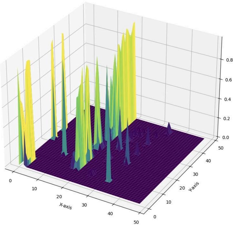
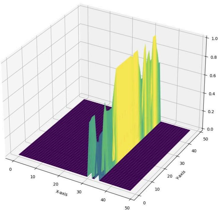 Fig. 4: Attention as a 3D Heatmap for Flood Semantic Segmentation Dataset at threshold 2.0 (without smoothing). Fig. 5: Attention as a 3D Heatmap for Flood Semantic Segmentation Dataset at threshold 0.4 (with smoothing).
Figures 6 and 7 explore the representation of attention values using 3D scatter plots, providing a distinct perspective on the attention distribution under varying levels of smoothing for the Large-Scale Dataset for Segmentation and Classification [38]. Figure 6 illustrates the attention values at a threshold of 0.9 (with light smoothing applied). It can be observed that the attention points are relatively sparse, with some clusters indicating areas of significant focus. However, higher threshold values limit the mechanism's ability to identify finer details in the distribution map. The light smoothing enhances the overall visual coherence, developing a stronger understanding of the focusing area where the fish is illustrated, yet it still retains some of the original fragmentation.
In contrast, Figure 7 presents the attention values at a threshold of 0.1 (with strong smoothing applied). Such an approach results in a dense interconnected scatter plot, where attention points are uniformly distributed across the attention region. The strong smoothing effectively blurs the boundaries between areas of high and low attention, creating a continuous representation of attention across the image data. Figure 7 highlights the strict relationships between different regions, making it easier to identify patterns that could have been missed in the original attention map's spatial inconsistency.
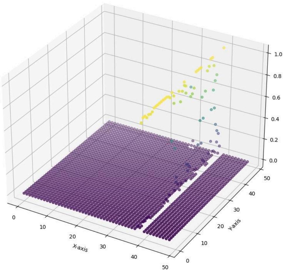 Fig. 6: 3D Scatter Plot for Attention Values at threshold 0.9 (light smoothing) for Large-Scale Dataset for Segmentation and Classification.
{"image_source":{"path":"images/af4c7b80e8de35c0dc9bd158b8711d12d6bd180b7b87da98d5cfd60c52fdbc98.jpg"},"content":"","chart_caption":[{"type":"text","content":"Fig. 7: 3D Scatter Plot for Attention Values at threshold 0.1 (strong smoothing) for Large-Scale Dataset for Segmenta- tion and Classification."}],"chart_footnote":[]}
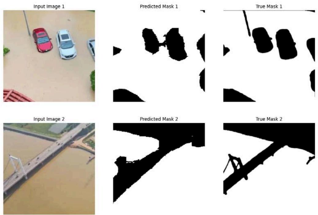
Figures 8 and 9 present the final predicted segmentation results for the Flood Semantic Seg-mentation Dataset [41]. Figure 8 illustrates the segmentation output at a threshold of 2.0 (withoutsmoothing applied), revealing the segmented images that are characterized by abrupt edges and fragmented regions. While some areas of interest are accurately captured, the lack of smoothing leads to a disjointed segmentation that does not effectively represent the underlying structural details in the spatial data.
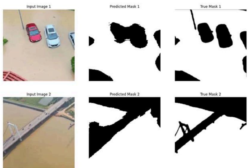 Fig. 8: Predicted Segmentation Result threshold 2.0 (without smoothing) for Flood Semantic Segmentation Dataset.
Smooth Attention_ Improving Image Semantic Segmentation
At the same time Figure 9 demonstrates the predicted segmentation mask at a threshold of 0.4 (with effective smoothing applied). The result with the Smooth Attention method achieves a more coherent and unified segmentation, having smoother transitions between the object boundaries. The application of smoothing constraint enhances the model's ability to capture complex shapes and relationships on the pixel-level, resulting in a segmentation mask that outlines detailed variation within the images.
We can see that the introduction of Smooth Attention notably improves the spatial distribution of the attention values within the attention map, helping the model to achieve better segmentation results. By incorporating a smoothness constraint, the Smooth Attention method encourages gradual changes in attention weights, which effectively mitigates the noise sensitivity problems with attention value distribution. We achieve the reduction of sharp transitions and foster a deeper understanding of spatial relationships of the image data.
 Fig. 9: Predicted Segmentation Result threshold 0.4 (with smoothing) for Flood Semantic Segmentation Dataset.
IV. CONCLUSION
To summarize, we introduce a new attention approach called Smooth Attention, designed to enhance the spatial coherence of attention maps in convolutional neural networks, particularly for vision tasks like image segmentation. Our experiments demonstrate that by incorporating a spatial distribution-aware smoothness enforcement mechanism, we improve the quality of the model's focus on relevant regions of the input images.
The Smooth Attention module effectively mitigates the complications of noisy attention patterns, resulting in smoother attention maps that still maintain the detail awareness inherent in traditional attention mechanism ideas. By leveraging Chebyshev distance to enforce spatial-aware smoothness, we achieve a balance between global and local attention, enhancing both the model's performance and interpretability.
Moreover, the adaptive nature of the learnable parameter and the tunable smoothness threshold provide the flexibility needed to tailor the mechanism to specific tasks and datasets. Such adaptability is essential for applications where varying degrees of spatial coherence are required, allowing to optimize the performance for the particular use cases based on the metrics results.
Future work will explore the application of Smooth Attention across other datasets and tasks, extending its use beyond image segmentation to other domains such as object detection and image captioning.
We believe that the Smooth Attention mechanism holds promise for advancing the interpretability and effectiveness of attention in convolutional neural networks for computer vision tasks. By addressing the challenge of spatial incoherence in attention maps, our approach paves the way for models that can better understand the complex visual data. We anticipate that this work will inspire further research in attention mechanisms in computer vision that prioritize interpretability and coherence, ultimately leading to more trustworthy AI systems in critical applications.
Disclosures
All the authors admit no conflict of interests.
Code, Data, and Materials Availability
All the datasets used are publicly cited and available. The code is submitted to GitHub storage and can be accessed publicly at: https://github.com/sparcus-technologies/Smooth-Attention-Improving-Image-Semantic-Segmentation
ACKNOWLEDGMENTS
The authors express gratitude to Sparcus Technologies Limited for providing computational resources for this research.
Conflict of Interest
The authors declare no conflict of interest.
Ethical Approval
Not applicable
Data Availability
The datasets used in this study are openly available at [repository link] and the source code is available on GitHub at [GitHub link].
Funding
This work did not receive any external funding.
References
Cite this article
Related Research



Special Issue
Launch a focused special issue to highlight research, emerging trends, and expert insights in your academic field.
