Algebra of Ecology

I. INTRODUCTION

When choosing one or another scientific approach, we proceed mainly from the goal - the closest possible description of the object being studied with its natural characteristics. This is precisely the approach that can be traced in most natural science research. But there is another option, namely: what the phenomenon being studied should ideally look like. This option makes it possible to consider the phenomenon under study not as an independent manifestation, but as a particular manifestation of the whole. In other words, the second option makes it possible to describe a holistic manifestation based on the study of its particular phenomenon. This approach considers the object under study in isolation from reality, i.e. an idealized version is studied. Naturally, such an approach will probably be formalized. Nowadays, such formalized options are increasingly in demand.

Modern scientific and technological progress is proof that it occurs on the basis of the emergence and establishment of abstract terms and paradigms. This atmosphere of development dictates the algebraization of the methodology of the problems being studied. This requirement of modern scientific and technological progress is caused by the development of artificial intelligence.

In a broader sense, algebra is understood as a section of mathematics devoted to the study of operations on elements of sets of arbitrary nature; in other words, abstract algebra is nothing more than a natural development of the axiomatic method, which deals with the study of operations performed on certain elements. The power and beauty of the ideas and methods of modern abstract algebra are widely recognized, and its scope of application is expanding so rapidly that there is sometimes talk of an "algebraic plague" that has engulfed not only mathematics but also other sciences (Fried, 1979). In the second half of the 20th century, the rapid development of the theory of elementary particles is a classic example of the application of methods of abstract algebra to solving fundamental problems in this area. The design of new types of technology and their use is unthinkable without the use of modern algebra methods, for example: electronic computers are designed on the principle of finite automata; methods of Boolean algebra are used in the design of electronic circuits; modern programming languages for computers are based on the principles of algorithm theory; computer search systems use set theory; in pattern recognition problems category theory is used; coding and decoding of information is carried out using methods of group theory, etc.

One of the important aspects of applying algebraic methods to the study of solutions to natural science problems is that it is not at all necessary to reduce the formulation of the problem to a purely mathematical one. This is a very important property of abstract algebra, since it allows one to use its methods in cases where the physical laws necessary for the transition from a physical problem to a mathematical one are not yet known. This is precisely the situation observed in the theory of elementary particles (quantum chromodynamics) (Lyubarsky, 1986; https://ru.wikipedia.org > wiki > Yang_Theory _—_Mi...).

Genuine, living, meaningful theoretical foundations of the problem being studied are born on the basis of a combination of abstract algebra and concrete problems. Algebraic studies of natural phenomena always reveal the internal and external harmony of the object being studied, and this is its beauty (Kline, 1984).

Any natural (physical, biological) and artificial (for example, agroecosystem) phenomena are based on the process of interaction of environmental factors.

Environmental factors can be viewed as various natural forces. If so, then the interactions of environmental factors can be viewed as interactions of various natural forces. Formalization and research of the interaction of environmental factors gave rise to many functions of survival rates of biological species (Gulamov, 1982; 1986; 1989; 1994; Gulamov, Pasekov, 1985; Gulamov, Fayziev, 1990, 1992; Gulamov, Khoshimov, 1997; Gulamov, 2006; 2012).

Algebraic studies of the set of functions of survival coefficients and information models made it possible to describe and identify certain algebraic patterns of ecological and information phenomena, for example: the minimum survival space; invariance of the elements of the set of functions of survival coefficients relative to each other; symmetrical relationships of ecological factors relative to each other; symmetrical relationships of ecological niches of species; formal description of the ecological field of survival and generalized operations of a set of information models.

The results of the study on a set of functions of survival rates of biological species, conducted by M.I. Gulamov in the period from 1982 to 2021, were the basis that made it possible to formalize them into a scientific monograph entitled "Algebra of Ecology". Naturally, this monograph does not cover all aspects of algebraic questions of ecology, these are only the first steps in the algebraization of ecology.

II. THEORETICAL BACKGROUND OF ECOLOGICAL ALGEBRA

2.1 Basic Concept

To formalize the interaction of environmental factors and the consequences of this interaction, we must first create its "idealized" version in order to be able to subsequently describe its formal model. For this purpose, it is necessary to introduce some basic concepts, which are the "building blocks" with which one can build its formalized model. Such basic concepts must meet two conditions: 1) they must reflect the main characteristics of the object being studied and 2) they must allow for a formal description of the phenomenon being studied. But we know that "bricks" are also made from a certain material. In our case, such material is the concept of the environmental factor. It follows from this that the basic concept that we will introduce should reflect the various aspects of the nature of the concept of an environmental factor.

From the above description and analysis of the concept of the environmental factor it follows:

1. An ecological factor is a certain force that changes according to certain patterns $f(A)$ and manifests itself as a condition or element of the environment $(A)$, capable of directly or indirectly influencing a living organism, at least at one of the stages of its individual development:

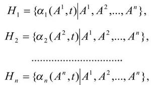
$f(A)$ where $A_i=\{a_i^1,a_i^2,\dots ,a_i^n\}$, $i=1,2,\dots$

1. Environmental factors are independent (meaning the absence of a linear relationship between factors) of each other:

1. A population is a minimal self-reproducing group of individuals of one species ( $N(t)$ ), which over a long evolutionary period inhabits a certain space, forms a genetic system and creates its own ecological niche.

2. Survivability is the ability of an organism or population to withstand the impact of environmental factors. This is, in percentage terms, the survival of an organism or the proportion of surviving individuals in a population.

3. Survival function is a quantitative expression of survival, characterizing the impact of an environmental factor $A_i$:

1. Optimality interval is an interval in the gradient of an ecological factor where the survival rate of an organism or individuals of a population is 100%:

1. The interaction of environmental factors can be represented as the interaction of the corresponding functions of survival rates:

1. Environment – formulating and determining the states of interacting environmental factors.

2. Ecological factors of the environment affect the organism or individuals of the population simultaneously and jointly:

Based on these basic concepts, research is conducted on the mechanisms of: survival of individuals in a population, interaction of environmental factors, calculation of ecological niches, as well as theoretical group research of the interaction of environmental factors.

2.2 Qualitative Study of Survival Mechanisms

Population analysis, Williamson (1975) notes, is one aspect of ecology and is currently made up of guesswork, intuition, and accumulated experience.

The discrepancy in the opinions of the majority of researchers on this issue and the lack of a clear picture of survival mechanisms have led to a revision of issues related to population dynamics. The purpose of this section is to study the mechanism of population dynamics based on the basic concepts that we have outlined above.

In natural conditions, environmental factors that determine the behavior of population dynamics are divided according to the nature of their impact into the following main groups:

1. external factors that do not depend on the size (density) of the population, characterized by their optimal values or optimal intervals in which the survival rate of individuals in the population is maximum (6th basic concept). Such factors include temperature, humidity, radiation, period of food availability, etc. (Gulamov, 1982; Gulamov, Pasekov, 1985; Shilov, 1985).

The qualitative behavior of the value of the survival function $\alpha (A,t)$ for the factors of this group is, for example, as in Fig. 1.

{"image_source":{"path":"images/9142d9d592fb677488d62ddaf551d7f99b61561f6b9ccae932f4ff447c7aa6c1.jpg"},"content":"","chart_caption":[{"type":"text","content":"Fig. 1: Qualitative Behavior of the Survival Function Value "},{"type":"equation_inline","content":"\alpha(A,t)"},{"type":"text","content":" in the Density-Independent Case"}],"chart_footnote":[]}

A quantitative dependence of this kind can be expressed, for example, as follows:

and in the case of the optimal value $a_1^{\ast }=a_2^{\ast }=a^{\ast }$. Where A is the density independent factor, $a_1^{\ast },a_2^{\ast }\in A$ are the boundary values of the optimal interval, $a(t)$ is the value of the factor A at time t, is the parameter responsible for the steepness of the survival function;

1. Factors whose effects change in direct, inverse or non-monotonic dependence on population density. Such factors include the density of the population itself, the density of parasites, predators, the intensity of the disease, etc. (Burov, 1968; Polivanova, Triselova, 1988; Semevsky, Semenov, 1982).

The qualitative behavior of the survival value for the factors of this group is, for example, as in Fig. 2.

Rice. 2: Qualitative behavior of the survival function value $\alpha (A,t)$ in the density-dependent case.

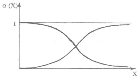
A quantitative dependence of this kind can be expressed, for example, as follows:

where $x(t-1)$ and $x(t)$ are the host population densities at times $(t-1)$ and t, respectively, $\theta$ and $\eta$ are parameters, $y(t)$ is the population density of parasites (predators) at time t (Viktorov, 1969; Kemp, Arms, 1989).

In addition, it is assumed that the survival rate of individuals in a population at any given moment in time is determined by the impact of a combination of factors that are density-dependent and independent (9th basic concept) (Viktorov, 1969; Gulamov, 1982; Shilov, 1985):

where $(A_1,A_2,...,A_n,t)$ is a set of density-dependent and independent factors; $\alpha (A,t)$ is the resulting survival rate, characterizing the impact of a complex of environmental factors.

From the optimal interval (3 basic concept) and the formal notation (4) (9 basic concept) it follows that under optimal conditions of density-independent factors $(\alpha (A,t)\to max)$, the dynamics of the population size is determined only by density-dependent factors, i.e. $N(t+1)=\alpha (\overrightarrow{X},t)\cdot N(t)$, where $X(t)=\{X_1,X_2,...,X_n,t\}$ is a set of density-dependent factors.

In the future, based on these hypotheses, we analyze all possible levels of population dynamics using thought experiments.

Depending on the combination of factors of the first and second groups, populations of different sizes may exist in different species (Odum, 1986 a, b; Ricklefs, 1979). Although there are different values of population size, population sizes are limited by a lower and an upper bound. This is expressed more voluminously by Odum (1986 b): "There are certain upper and lower limits to population sizes that are observed in nature or that could theoretically exist for an arbitrarily long period of time."

The impossibility of analyzing the entire spectrum of population levels forces us to select among them a set of levels, the analysis of which will give an approximate continuous change in the population dynamics as a whole. Based on these considerations, the spectrum of population size levels can be conditionally divided into three levels:

1. lower maximum permissible level; 2) average level; and 3) upper maximum permissible level.

Based on the above hypotheses, the population dynamics can theoretically be represented in the form of a graphical model in Fig. 3.

{"image_source":{"path":"images/d20af6000087f6e700c58a9c90ddf54204df0f3adbf50ae3a356371e0b08f6f7.jpg"},"content":"","chart_caption":[{"type":"text","content":"Fig. 3: Hypothetical Model of Population Dynamics"}],"chart_footnote":[]}

The lower permissible limit (Fig. 3, range I) is determined by the dominance of the role of one of the groups – density independent ( $\alpha (A,t)\to min$ ) or dependent ( $\alpha (X,t)\to min$ ) factors. At this level, the species adapts and acquires certain traits that increase the survival rate and fertility of individuals under unfavorable living conditions. As E. Pianka (1981) explains, under such conditions animals experience weak competition and are subject mainly to r-selection. In such environmental conditions, the lower maximum permissible level is a potential basis for the transition to the average level of abundance.

At the average level (Fig. 3, range II), the regulation of numbers below the saturation level (Fig. 3, range II, a) is determined by density-dependent and independent factors (Rasnitsyn, Volkova, 1982). This density level is characterized by the same values of the survival function for both groups of factors $(\alpha (A)\approx \alpha (X))$. This combination of factors corresponds to the condition of the ecological optimum of I.A. Shilov (1985) - "this is the most favorable combination of all (or at least leading) ecological factors, each of which most often deviates somewhat from the physiological optimum." This combination of two groups of factors leads to stabilization of the population at this level, i.e. the smallest fluctuations in population occur within this level. $N(t)=N(t-1)=N^{\ast }$. In addition, a conditional stationary state is possible, that is, preservation over a short period of time. $\alpha (x^{\ast })=\exp (-\theta )$ This state generates a stationary density-dependent factor, the value of which is characterized by (3). Such a stationary density-dependent factor is the cause of the violation of the stationary state at the next t+1 moment in time, which leads to an oscillatory regime. $\alpha (A,t)$ Deviation of the value from the average value ${\alpha }_{av}(A,t)$ leads to a decrease or increase in the number. When decreasing, the number falls into the lower maximum permissible level, which was discussed above, and when increasing, into the saturation zone (Fig. 3 range II, b), which is a prerequisite for moving to the upper permissible level (Fig. 3 range III). In the saturation zone (Fig. 3 range II, b), provided that the values $\alpha (A,t)$ are close to the physiological optimum, species can realize their maximum possible fertility (Isaev, Khlebopros, 1973).

This behavior of the species in the saturation zone leads to fluctuations in their numbers.

The upper maximum permissible level (Fig. 3 range III) of the population is reached when $\alpha (A,t)\to max$, and the population level is in the saturation zone. Under such conditions, population fluctuations occur. This in turn increases the influence of density-dependent factors, that is $\alpha (X,t)\to min$, which leads to a decrease in the population level.

The mental experiments we conducted to study the spectrum of population size levels allow us to draw the following conclusion:

where ${\alpha }_{av}(A,t)$, $N_{av}(t)$, ${\alpha }_{av}(X,t)$ are average values.

From these relationships it follows: firstly, the levels of population dynamics are determined by density-dependent factors in conditions when $\alpha (A,t)\to max$ the population size is at the upper limit of permissible level, in other cases the main role is played by density-independent factors; secondly, one-sided conditionality is obvious $\alpha (A,t)\Rightarrow \alpha (X,t)$, that is, behavior $\alpha (X,t)$ is determined by the very nature of the function $\alpha (A,t)$. Lindstrom Research J. at al (2001) is proof of this.

To summarize, it can be said that the decisive role in the dynamics of the population size is played by the factor for which the values of the survival function are closer to the minimum (Odum, 1986 b).

2.3 Interactions of Environmental Factors

Environmental factors affect the body simultaneously and jointly (1.1. 9 basic concept).

In studying the combined impact of environmental factors on a particular biological object, all factors that can be measured are taken into account. But here the main emphasis is not on identifying the main factors and studying their impact separately on the dynamics of the population, but on the interactions of factors with each other and determining the resulting, joint impact on the dynamics of the object (Sharov, 1985, 1989; Iogansen, 1964; Kemp, Arms, 1989; Gulamov, 1994, 1996).

In order to more clearly imagine the interaction of environmental factors with each other, we will use Hutchinson's concept of a fundamental ecological niche. He believed that an ecological niche should be defined by taking into account the entire range of physical, chemical, and biological environmental variables to which a given species must adapt, and under which a given population lives and renews itself indefinitely. Ideally, each such variable can be viewed as a gradient along which each species has its own range of activity or stability (Bigon et al., 1989; Giller, 1988; Hutchinson, 1991). n A comprehensive analysis of environmental variables (factors) corresponds to the consideration of an ecological niche as a certain set in n a -dimensional space.

If each such variable is considered as a gradient, on which each species has its own range of survival, then the corresponding n-dimensional hypervolume (ecological niche) of the species can be represented as a certain n-dimensional hypervolume of its survival. Then the problem of the complex impact of environmental factors on the survival of individuals in a population can be considered from the point of view of n the -dimensional hypervolume of species survival, and the complex impact of factors should be understood as a non-trivial form n of -dimensional set, different from the traditional parallelepiped of Hutchinson's fundamental niche.

Let us assume that we know some combination of environmental factors - $A^1,A^2,\dots ,A^n$ at time $t$ and the corresponding survival functions ${\alpha }_1(A^1,t),{\alpha }_2(A^2,t),\dots ,{\alpha }_n(A^n,t)$, which we will consider to be continuous monotone curves defined in the corresponding one-dimensional spaces of factors and displaying them in the segments [0,1](5th basic concept). The explicit form of these survival functions is presented above (Gulamov, 1982, 1989).

Let us assume that the factors are independent of each other (2nd basic concept), then the survival functions under consideration as functions over the entire space of factors generate "cylindrical" surfaces (the generators of which are parallel to the space of the remaining $(n-1)$ factors):

Where $A^i\in R$, $i=\overline{1,n}$. In this case, the interaction of environmental factors can be understood as the intersection, product, union or sum of these cylinders ( $H=\bigcap _n{H}_{i}H=\prod _n{H}_i,H=\bigcup _n{H}_{i}orH=\sum _{i=1}^n{H}_i$ ), and the measure of the joint impact of the environment is the hypervolume of this intersection of the product, union or sum H. H clearly, this is the minimum or maximum possible hypervolume of survival at time t (Gulamov, 1991; Gulamov, Logofet, 1997). The survival value at any point on the surface of the formed hypervolume (H) at time t can be written, following the theory of fuzzy sets, as follows:

Following the above reasoning, given in the section "Factorial Theory" and Liebig's principle, we can say that the measure of the joint influence of the environment is the hypervolume formed by the intersection of "cylindrical" surfaces $-H=\bigcap H_i$

Thus, each point on the surface of such a hypervolume is determined by the minimum values of the survival function for individual factors, i.e., according to the Liebig principle. An example of the minimum survival hypervolume is the one considered in the work of G.E. Zaikova and others. (1991), the result of experimental observation is a diagram of the dependence of fish fry survival on the concentration of calcium (Ca) and aluminum (Al).

Let us now turn to the situation when it is necessary to take into account the nature of the interaction of environmental factors. Analysis of the works of Tingey and Reinert (Tingey, Reinert, 1975), Shin and others. (Shinn and al., 1976), Howe et al. (Hau and al., (1977) and Raneckles (1988) show that pollutants in atmospheric air are present in various combinations, as a result of which the effect of their combined or sequential exposure on individuals of a population differs from the effects of exposure to a single substance. Such combined effects can lead to antagonistic, additive, or synergistic effects (Streffer, Bucker, Consier, 2003).

1. Additivity - the effect of a mixture (i.e. the summation of individual substances) differs from the effect of the substances separately included in the mixture.

2. Synergism is the effect of a mixture of several substances that is greater than the effect of the sum of the effects of each of them.

3. Antagonism - the effect of the mixture is less than the combined effect of each substance.

(n) in the aggregate must necessarily be present. If we denote the survival function for each environmental factor in three cases of their interaction as: ${\alpha }_i(A^i,t)$ with additivity, ${\alpha }_i(A^i,t,n)$ with synergism, ${\alpha }_i(A^i,t,n)$ with antagonism, $i=1,\dots ,n$, then the resulting values of the survival function in all considered types of interaction must satisfy the inequality

In all three cases considered, the resulting values of the survival function are determined similarly (8 in the case of intersection), but the "cylindrical" surfaces of the independent case must give way to surfaces of a more complex nature – the corresponding families of single-factor survival functions, covering a known variety of other factors.

Based on the resulting values of the survival function (8), one can judge the stability of the nature of the interaction of environmental factors. For example, when $\alpha (\overrightarrow{A},t)\to 1$ the considered nature of the interaction of environmental factors is stable, but $\alpha (\overrightarrow{A},t)\to 0$ unstable.

Relation (9) can be used to verify the obtained approximations.

Based on the resulting values of the survival function (8), one can judge the stability of the nature of the interaction of environmental factors. The closer $\alpha (\overrightarrow{A},t)\to 0$, the more stable the interactions of environmental factors according to the given nature of interaction, the closer $\alpha (\overrightarrow{A},t)\to 0$, the less stable.

Taking into account the above-mentioned effects of interaction of environmental factors in the expressions of the exponents of the survival functions, given in the section "Qualitative study of the mechanisms of population survival", it is possible to write in a more general form, for example for i the -th factor: $\exp (-\gamma \mathrm{\Delta }{a}_i(t))$.

Depending on the type and value of the factor $A^i(t)$ (whether it is optimal or not), $\mathrm{\Delta }{a}_i(t)$ it can be: with a difference, equal to zero (0), or a ratio. Taking into account the type of interaction and the number of environmental factors, the following is clearly $\exp (-\gamma \mathrm{\Delta }{a}_i(t))$ evident:

1. with additivity $\exp (-\gamma \mathrm{\Delta }{a}_i(t))$,

1. in synergy $\exp (-\gamma \mathrm{\Delta }{a}_i(t)\cdot n)$, (10)

2. in antagonism $\exp (-\gamma \mathrm{\Delta }{a}_i(t)/n)$.

A comparative analysis of the factorial theory and the theory of interaction of environmental factors shows:

i.e. the approach we propose to determine the resulting survival function may be equal to or overestimated relative to the multiplicative form and strictly less than relative to the additive form of recording (Gulamov, 2004).

2.4 Formal Definition of an Ecological Niche

The approach to describing a niche proposed by Hutchinson (1959, 1978, 1991) has received the greatest number of adherents. Using set theory, he formalized the problem and defined a niche as the set of conditions under which a population lives and reproduces itself. Hutchinson called the entire set of optimal conditions under which a given organism can exist and reproduce itself a fundamental niche.

Hutchinson viewed a fundamental niche as a region of multidimensional space, or hypervolume, within which environmental conditions allow a population to persist indefinitely. Therefore, a fundamental niche is a hypothetical, imaginary niche in which the environment is optimal for individuals in a population and in which it does not encounter "enemies" such as competitors and predators. In contrast, the actual range of conditions for the existence of an organism, which is always less than or equal to the fundamental niche, is called the realized niche.

The realized niche of most organisms changes in time and space depending on changes in the physical and biological environment. Temporal changes in a niche can be considered at two levels: 1) at the level of short-term changes (on the scale of ecological time), usually occurring during the life of an individual or, at most, several generations; 2) at the level of long-term changes occurring on the scale of evolutionary time and affecting many generations. Thus, the realized niche can be considered as a constantly changing subset of the fundamental niche or, in terms of multidimensional space, a pulsating hypervolume, which is limited by the hypervolume corresponding to the fundamental niche (Pianka, 1981).

The dimensions of the multidimensional space describing the environment are the gradients of environmental factors. If the environment is described by n factors, then the ecological niche can be described in terms of the corresponding n -dimensional space (Gulamov, 2002).

For example, in the case of inactive factors, the ecological niche can be represented as follows. Let for each factor $X_j$ of the ecological space $E_n$ there exist a tolerance interval of the population $[x_{j1},x_{j2}]$ such that the well-being function $f_j(X_j)$ for the factor $X_j$ is equal to one inside this interval and zero outside it. The set of all points $(x_1,x_2,...,x_n)n$ -dimensional space, all coordinates of which are within the corresponding tolerance intervals, i.e. satisfy the conditions

forms an n -dimensional parallelepiped

with sides parallel to the coordinate axes $X_1$, $X_2$,..., $X_n$ n-dimensional space. For example, for the case n = 3, this is a normal three-dimensional parallelepiped

Of course, in the case of dependent factors, the n -dimensional region corresponding to the ecological niche may have a more complex configuration.

Hutchinson's definition of a niche had a revolutionary impact on the development of ecological theory. This is connected, firstly, with the fact that Hutchinson's niche can be described in a formal language and operated with mathematically. Secondly, the niche was determined by him, first of all, based on the properties of organisms and their relationships in the community. At the same time, Hutchinson emphasized that in the process of evolution of organisms or communities the situation can change, and a niche previously occupied by one species can be divided between several more specialized species (Hutchinson, 1978; Nikolaikin et al., 2003). Thirdly, the concept of the fundamental niche developed by Hutchinson was of great importance for the development of the concept of the ecological niche. The fundamental niche is sometimes called the pre-competitive or potential niche, and the realized niche is called the post-competitive or actual niche. This approach gave rise to a direction associated with the predominant study of the role of competition in the division of environmental resources. These works include (MacArthur, 1961, 1968, 1970, 1972; MacArthur, Levins, 1967; MacArthur, Pianka, 1966, MacArthur, Wilson, 1967).

A careful analysis of the definitions of ecological niche presented by Grinnell, Elton, Odum, Pianka and Hutchinson shows that their essence coincides. The differences lie rather in the use of different terminology, and also in the fact that they reflect different stages in the development of this approach, culminating in the definition given by Hutchinson.

However, although the modern concept of ecological niche is based on the multidimensional niche model developed by Hutchinson, ecological niche has increasingly come to be identified with the spectrum of resource use along just one or more of the most important (or most easily measured) dimensions of the niche. The reason for this is that the model of a niche as an n -dimensional hypervolume is too abstract. Usually, most parameters are given implicitly and are defined only qualitatively; for example, the explicit form of the well-being function is not defined. When the number of environmental factors is more than three, description (13) loses its visual meaning, etc. Therefore, usually several of the most important dimensions are distinguished, along which, one way or another, the division of resources and the divergence of species into niches occurs: food, space and time.

From the above it follows that the concept of an ecological niche is given mainly a qualitative meaning and this approach is difficult to apply to solving applied problems. True, the works of Yakhontov (1969), Pianka (1981), Odum (1986b), Giller (1988) provide examples of the application of the concept of an ecological niche to the solution of a number of specific ecological problems concerning the size of a habitat, the rate of population growth, fitness, r- and K - selection, time distribution, morphological features (such as, for example, the thickness and length of a bird's beak), etc. However, all these applications are qualitative in nature, i.e. they lack quantitative assessments that could be used for comparative analysis of ecological niches of different species.

True, such problems at present, in the context of the rapid development of information technology, can be solved quantitatively. As an example, we can consider the works:

Peterson (2001) considers predicting the geographic distributions of species based on ecological niche modeling for the purpose of studying biodiversity. This study mainly uses the ecological niche models of species development based on artificial intelligence algorithms, GARP and GIS and projects them onto geography to predict species.

Sibly and Hone (2002) consider the formation of an organism's ecological niche from the resulting impact of environmental factors and the rate of population growth. In this paper, the authors make more realistic conclusions that an ecological niche is the result of the interaction of a complex of environmental factors and the rate of population growth. Although the authors do not specify the "resulting impact" of environmental factors.

Anderson et al. (Anderson at al., 2002) study the geographic distribution of mice (Heterde australis and H. anomals) in South America by constructing their ecological niches based on GIS modeling. The basis of such modeling is the idea that the matrix of a complex of favorable factors in relation to the species under consideration is formed and then checked using certain methods, a comparative analysis is made with these geographic locations. Although the results of the study do not confirm the actual situation, they nevertheless provide an opportunity and are a good basis for testing this kind of scientific hypotheses through field and laboratory research.

Hirzel et al. (Hirzel at al., 2002) consider ecological niche as a factorial analysis. According to Hutchinson's concept, an ecological niche is constructed in the area of multidimensional ecological factors, the distribution of neighborhoods, where the distribution of varieties is observed according to a set describing the entire area of study. The first thing that will be given is the fact of maximizing the probability of densification of a variety, defined as the ecological distance between the optimal densifications of varieties and the average ecological niche within the areas under consideration. This, in turn, provides a habitat suitability map.

Lim et al. (Lim, Paterson, Engstrom, 2002) construct an algorithm for modeling a sustainable ecological niche for mammals in Guyana. This model is used to solve real environmental problems such as the distribution of diversity in the open spaces and forests of Guyana. In this work, genetic algorithm for rule set prediction (GARP) is used.

Peterson et al. (Peterson, Ball, Cohoon, 2002) test the utility of the genetic algorithm rule set prediction (GARP) modeling program for ecological niche modeling to make accurate geographic distribution predictions for 25 Mexican bird species. The authors conclude that the trial was a success (78-90%), indicating that ecological niche modelling approaches such as GARP provide a promising tool for investigating a wide range of questions in ecology, biogeography and conservation.

The above-mentioned modern works on modeling ecological niches are mainly practical in nature and differ from the work of V.V. Yakhontov (1969), Yu. Odum (1986), E. Pianka (1981) and P. Giller (1988) in that, thanks to the capabilities of modern computers, they can operate with a large number of ecological factors. The presented modern models of ecological niches are mainly based on Hutchinson's multidimensional ecological niche. Basically, the principle of operation of these models of ecological niches (GIS, GARP) is based on the method of matrix comparison, i.e. the data table for a species (organism or population) is compared with geographic data tables. Based on this comparison, appropriate conclusions are made regarding distribution, biodiversity, etc.

The theoretical basis of the presented works on modeling ecological niches remains the same at the level of Hutchinson's multidimensional ecological niche.

Although the work of E.I. Khlebasolov (1999) was published several times earlier than the above-mentioned modern works, nevertheless his conclusions have not lost their relevance: "Despite the significant volume of factual data and theoretical generalizations, it has not yet been possible to fully determine the essence of understanding ecological niches. Modern models based on Hutchinson's multidimensional niche theory attempt to understand the nature of species interactions in a community by measuring the width and degree of niche overlap in one or more of the most important indicators. At the same time, little attention is paid to the study of the properties and parameters of the niche itself. Therefore, the modern approach contains a number of limitations that hinder the further development of niche theory and understanding of the mechanisms of formation and functioning of ecosystems. This serves as a reason for a pessimistic assessment of the state of research in the field of community ecology and encourages biologists to search for alternative approaches to studying the problem of niches."

2.5 Generalization of Hutchinson's Definition

An ecological niche is defined by Hutchinson as a set of environmental factors in space. In turn, one of the ways to define a set in space is to use characteristic or indicator functions (Mathematical Encyclopedic Dictionary, 1988). The indicator of a set is a function that is equal to one at points in the set and zero at points that do not belong to the set. In fact, such an indicator for one dimension is the above -mentioned binary (i.e. taking only two values) well-being function $h_j(X_j)$ for factor $X_j$. Fig. 4 illustrates this situation (Gulamov, Terekhin, 2004).

{"image_source":{"path":"images/628fb73d791c72c3a9e1dcf2c4c3b6367bcc091bd3368b455d3a29240a8b2493.jpg"},"content":"","chart_caption":[{"type":"text","content":"Figure 4: An example of a one-dimensional Hutchinson ecological niche "},{"type":"equation_inline","content":"[X_{j1}, X_{j2}]"},{"type":"text","content":" given by a binary (taking only two values) indicator function of well-being "},{"type":"equation_inline","content":"h_{j}(X_{j})"}],"chart_footnote":[]}

If the environment is described by two factors $X_j$ and $X_k$, then the indicator function of well-being will be a function of two variables $-h_{jk}(X_j,X_k)$. In Fig. 5 shows an example of a two-dimensional indicator function for a situation where factors $X_j$ and $X_k$ do not interact within the boundaries of their one-dimensional niches, i.e., a one-dimensional niche for factor $X_j$ does not depend on the value of factor $X_k$, as long as its values do not go beyond the niche for this factor, and a one-dimensional niche for factor $X_k$ does not depend on the values of $X_j$ within their niche boundaries. In this case, the two-dimensional indicator function (and, consequently, the niche itself) can be reconstructed from the known one-dimensional indicator functions of the non-interacting factors $X_j$ and $X_k$ either by multiplying them or by taking their minimum, i.e.

or

which leads to the same result, illustrated in Fig. 5. We cannot, however, say that in this situation the interaction of factors is completely absent: if the value of one of the factors goes beyond the boundaries of its niche, then the one-dimensional niche for the other factor becomes an empty set.

In more complex situations, the one-dimensional niche for factor $X_j$ may depend on the value of factor $X_k$, and the one-dimensional niche for factor $X_k$ - on the value of $X_j$. So, in Fig. 6 shows the situation when one-dimensional niches by factor $X_j$, corresponding to two different values $x_{ka}$ and $x_{kb}$ of the factor $X_k$, do not even overlap. To find a two-dimensional niche in such cases, one must know either one-dimensional niches by factor $X_j$ for all values of factor $X_k$, or one-dimensional niches by factor $X_k$ for all values of factor $X_j$.

{"image_source":{"path":"images/1b6a5ae56d419094fc6b6f6ed55b6a823e1cc5dd9c7f435064bad06611fd3695.jpg"},"content":"","chart_caption":[{"type":"text","content":"Figure 5: An example of a two-dimensional ecological niche of Hutchinson, given by a binary indicator function of well-being "},{"type":"equation_inline","content":"h_{jk}(X_{j}, X_{k})"},{"type":"text","content":", equal to one above the shaded area and zero outside this area (the case of factors not interacting within the boundaries of the niches)"}],"chart_footnote":[]} {"image_source":{"path":"images/bb93a86a89b60862ea5639fc34731d35549d2aff03b2d50a182479e133d2c1b0.jpg"},"content":"","chart_caption":[],"chart_footnote":[]}

Figure 6: An example of a two-dimensional Hutchinson ecological niche given by a binary indicator function of well-being $h_{jk}(X_j,X_k)$ equal to one above the shaded region and zero outside this region (the case of significantly interacting factors)

P.A. Zade (1976) generalized the concept of a set by introducing the concept of a fuzzy or blurry set (fuzzy set). If in the classical sense a set can be defined by a binary indicator function, which for each point in space indicates its membership or non-membership in the set, then a fuzzy set is defined by an arbitrary non-negative indicator function, the value of which at any point characterizes the degree of membership of this point in the set. For example, the probability density function of a random variable can be considered as a special case of such an indicator function.

By replacing the term "set" in Hutchinson's definition of an ecological niche with a "fuzzy set", i.e. allowing non-binary well-being functions as indicator functions, we obtain a definition of a generalized, one might say, "fuzzy", ecological niche. This generalization seems to us as natural as it is to use softer, gradual functions of well-being instead of contrasting binary ones. It is obvious that fuzzy ecological niches can more adequately describe real situations. In Fig. 7 shows an example of a one-dimensional non-binary indicator function, which is taken as the density function of the normal distribution.

In Fig. 8 gives an example of a fuzzy ecological niche defined by a non-binary indicator function of well-being $g_{jk}(X_j,X_k)$ for the case of multiplicatively interacting factors $X_j$ and $X_k$. The degree of belonging of points of space to a niche, i.e. the magnitude of the values of the indicator function, is represented by the saturation of the gray color. The values of the function $g_{jk}(X_j,X_k)$ are obtained by multiplying the values of two one-dimensional indicator functions, which are the normal distribution density functions $g_j(X_j)$ and $g_k(X_k)$.

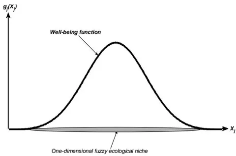
$[X_{j_1},X_{j_2}]$ defined by a non-binary indicator function of well-being $g_j(X_j)$ (the density function of the normal distribution is taken)

Figure 8: An example of a two-dimensional fuzzy ecological niche defined by a non-binary indicator function of well-being $g_{jk}(X_j,X_k)=g_j(X_j)\times g_k(X_k)$ (the case of multiplicatively interacting factors). The magnitude of the values of the function $g_{jk}(X_j,X_k)$, characterizing the degree of belonging of points in space to the niche, is represented by the saturation of the shading.

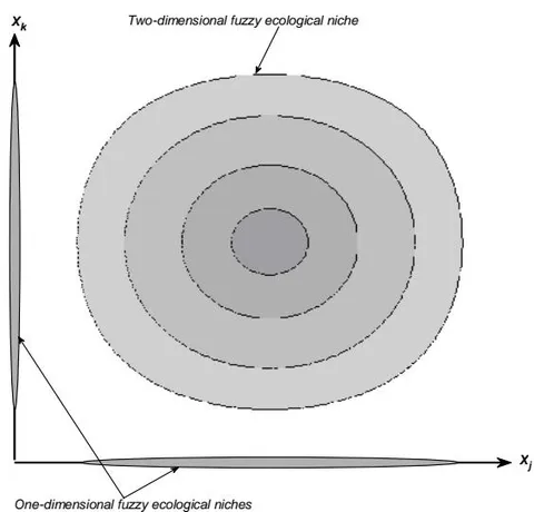
In Fig. 9 shows another example of a blurred ecological niche. In this case, the two-dimensional indicator function of well-being $g_{jk}(X_j,X_k)$ is obtained by taking the minimum of the values of two one-dimensional indicator functions $g_j(X_j)$ and $g_k(X_k)$ (this type of interaction of factors can be called limiting). Unlike Fig. 8, where the two-dimensional indicator function has a bell-shaped form, and its level lines are concentric circles or ellipses, in the situation of Fig. 9 The two-dimensional indicator function resembles a square or rectangular pyramid, and its level lines are squares or rectangles.

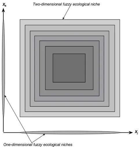
$g_{jk}(X_j,X_k)=min\{g_j(X_j),g_k(X_k)\}$ (the case of non-interacting factors). The magnitude of the values of the function $g_{jk}(X_j,X_k)$, characterizing the degree of belonging of points in space to the niche, is represented by the saturation of the shading.

2.6 Practical Aspects of using the Apparatus of Fuzzy Ecological Niches

Using the above definition of a blurred ecological niche and introducing additional hypotheses about the nature of the interaction of ecological factors (Gulamov, 1994; Gulamov, Logofet, 1997), one can obtain a practically working apparatus for the quantitative description of the environment.

Let $g_k(X_k,x,y,t)$ is a one-dimensional survival function of a certain species with respect to factor $X_k$, $k=1,2,...,n$, at a geographic point $(x,y)$ at time $t$. In the case of simple interactions of multiplicative or limiting type, the multivariate survival function can be reconstructed from one-dimensional functions.

Let's consider the limiting interaction. In this case, the multivariate survival function describing the joint action of factors will be a surface over the space of all factors, defined by the formula

i.e. each point of the multidimensional survival surface is determined by the minimum survival for all factors, i.e. according to the Liebig principle (Odum, 1986 b). As an illustrative example, we can refer to the results of an experimental determination of the dependence of fry survival on the concentrations of calcium (Ca) and aluminum (Al), given in the work of G. E. Zaikov et al. (1991).

To carry out calculations to find fuzzy niches, we created a special computer program (Gulamov, 1982; 1989). By setting the values of factors with a certain time step at different points of the area, it can be used to obtain the dynamics of a niche for a given area over a certain time interval. Some of its practical applications are described in (Gulamov, Logofet, 1997; Gulamov, 1995).

Thus, the proposed approach to formalizing an ecological niche makes it possible to find real ecological niches of populations and species and allows for their comparative analysis for different biological objects. In addition, it allows us to solve a number of problems in applied ecology, such as predicting the distribution of a species across its range, ecological zoning of a region relative to the values of environmental factors of interest to us, and obtaining ecological assessments of the area.

III. GROUP-THEORETIC RELATION OF THE SURVIVAL RATE FUNCTION

The application of the group-theoretical approach to the study of biological phenomena is caused by some features of these problems. What are these features?

Before answering this question, it is necessary to present those features of physical problems that served as the basis for the application of group-theoretical approaches in the study of solutions to these problems. Such a feature is the symmetry properties of physical problems. For example, the symmetry of space and time plays a fundamental role in physics. Its manifestations are varied. In its most general form, it is expressed in the fact that all inertial reference systems are physically equivalent. It follows from this that all physical laws have the same form in all non-rational reference systems.

To apply the methods of group theory to the study of solutions to a particular physical problem, it is not at all necessary to bring the formulation of the problems to a purely mathematical level. This is a very important property of group theory, since it allows one to use its methods even in cases where the physical laws necessary for the transition from a physical problem to a mathematical one are not yet known. This is precisely the situation that is currently observed in the theory of elementary particles (Lyubarsky, 1986).

Now let's answer the question posed above. This is, firstly, the identical symmetrical structure of the gene structures of most living beings; secondly, the presence of clear classification structures (taxonomy) in biology, which reflect the relationships between organisms, and, thirdly, the predominantly qualitative, rather than quantitative, nature of the concept of biological patterns. All these features, such as symmetry, classification and the qualitative nature of biological concepts, may be the features that would allow the application of the group-theoretical approach to the study and solution of a number of biological problems.

Applying the above to the problem we are studying, we can note, firstly, the presence in the general case of only qualitative characteristics of the survival function (see Fig. 1 and 2), and, secondly, the study of the relationships between two types of factors (density-dependent and independent) of the survival of individuals in an insect population showed that the survival functions for these types of factors can differ from each other by only one or two parametric transformations (parameters mean slope and shift). All this speaks to the entirely appropriate application of the group-theoretical approach to studying the solution to the problem of interaction of environmental factors (Gulamov, Fayziev, 1990; 1992).

3.1. Group-Theoretical Study of the Survival Rate Function

This section is a study of the relationship between two types of density-dependent and density-independent factors with respect to their survival function using the mathematical apparatus of group theory. This approach does not seek to identify any one main dominant type of factor, but rather attempts to identify the relationship between these two types of factors. We proceed from the assumption that the cause of fluctuations in population size is all possible combinations of density-dependent and independent factors. Viktorov (1971) said it very well on this matter: "...it is more likely that an analysis of the factors of population dynamics can help to clarify the causes of fluctuations in productivity than that a quantitative characteristic of the flow of matter and energy through a population will provide the key to understanding the causes of its dynamics."

In a qualitative study of the mechanisms of population survival, we came to the conclusion: the behavior of the survival function as a function of density-dependent factors $(\alpha (X))$ is determined by the very nature of the determination of the survival function as a function of density-independent factors $(\alpha (A))$.

{"image_source":{"path":"images/bde1769317425de93984b4312acf40a75e7562d16a02a1c1f1fbee0bcee54c64.jpg"},"content":"","chart_caption":[],"chart_footnote":[]} {"image_source":{"path":"images/f03f7b0dffd3c14377b86901392140499c66a2d51b451ef21c7c782ede540977.jpg"},"content":"","chart_caption":[],"chart_footnote":[]}

{"image_source":{"path":"images/e41022018bf5e1f6ea7824ebe461c985dd615070a617bda37445e1e277c62332.jpg"},"content":"","chart_caption":[],"chart_footnote":[]} {"image_source":{"path":"images/e47a0c617994599ac98ab42c58cadf1f496ece1c1f4f2d4214b5425cbeaa56f5.jpg"},"content":"","chart_caption":[],"chart_footnote":[]}

{"image_source":{"path":"images/a9aab16ad7ab26abad0759de95f545543e252281450a4e284bcb6d8b11f564c2.jpg"},"content":"","chart_caption":[],"chart_footnote":[]} {"image_source":{"path":"images/30a7db75f4f71192c1f280f076b96dce14ecc3e12d3cd919d55957155de8c77c.jpg"},"content":"","chart_caption":[{"type":"text","content":"Rice. 10: Qualitative behavior of the survival function under the operations translation, rotation "},{"type":"equation_inline","content":"\pi"},{"type":"text","content":" and transformation "},{"type":"equation_inline","content":"1 - \alpha(z)"},{"type":"text","content":"."}],"chart_footnote":[]}

To analyze the relationship between the two types of factors described above, we will proceed as follows. We abstract from specific types of factors, replacing them with some generalized set of factors Z, the components of which are density-dependent and independent factors:

For simplicity, we will first consider the values of the survival function $\alpha (k\cdot z)$ with the steepness parameter k=1 (i.e.) and for all possible values of z, where $z\in Z$. $\alpha (z)$ Let some behavior of the survival function ( $\alpha (z)=e$ ) of the type shown in Fig. 10 be given. $f(z)$ 10 a, we will denote it by.

$f(z)$ By shifting (translating) to the point $z^{\prime }$ we obtain: $f(z-z^{\prime })=x$ (Fig. 10b), then we rotate $\pi$ around the axis (perpendicular to the axis Z) passing through the points $z^{\prime }$, and obtain: $f(z^{\prime }-z)=A$ (Fig. 10c), i.e. mirror reflection of the function $f(z-z^{\prime })$. Let's perform transformations $1-\alpha (z)$ on the function $f(z^{\prime }-z)$ and obtain: $1-f(z^{\prime }-z)=B$ (Fig. 10g). $1-f(z^{\prime }-z)$ for the function, we once again apply the rotation operation by $\pi$, as a result we get $1-f(z-z^{\prime })=Y$ (Fig. 10d). $1-f(z-z^{\prime })$ Shifting to the origin, $1-\hat{f}$ we get $1-f(z)=C\cdot 1-f(z)=\hat{f}$. Once again transforming, as $1-\stackrel{▽}{f}$, we obtain $1-(1-f(z))=f(z)=e$ (Fig. 10a). $\alpha (z)$

All possible options $\alpha (z)$ shown in Fig. 10, were obtained from the state (Fig. Z 10 a) by successive action of the operation: shift (translation) along the abscissa axis $f(z)$, rotation by $\pi$, relative to (perpendicular to the axis Z), passing through some fixed point $z^{\prime }$ and transformation $1-\alpha (z)$.

Let T denote the set of monotone functions (such as in Fig. 10), mapping R into the segment [0,1], and let S(T) be the symmetric group of the set T, i.e. the group of all one-to-one mappings of T onto itself, where the product of two mappings $\phi$ denotes $\psi$ their superposition.

For each $z^{\prime }\in R$ denote by $G(z^{\prime })$ the subgroup of S (T) generated by the set $P(z^{\prime })=\{x(z^{\prime }),y(z^{\prime }),a(z^{\prime }),b(z^{\prime }),c\}$ (the elements x, y, a, b, c are X, Y, A, B, C respectively, and note that the element does $c\in P(z^{\prime })$ not $z^{\prime }$ depend on), where the elements of $P(z^{\prime })$ act on the set T as follows (the result of the action of the element $g\in S(T)$ on the function $\phi \in T$ is denoted by ${\phi }^g$ ):

It is easy to verify that from formulas (14) it follows that if $z^{\prime }\ne 0$, That $a^2(z^{\prime })=b^2(z^{\prime })=c^2=e$, and the elements $x(z^{\prime })$ and $y(z^{\prime })$ have an infinite order, if then $z^{\prime }=0$, it is obvious that $x^2(z^{\prime })=y^2(z^{\prime })=e$.

Let $z^{\prime }\ne 0$. the study of the structure of the group $G(z^{\prime })$ show that in terms of generating and defining relations $G(z^{\prime })$ it has the following form:

Let us denote by $G$ the subgroup of the group $\mathbf{S}(\mathbf{T})$ generated by the set $\{G(z^{\prime })|z^{\prime }\in \mathbf{R}\}=Q$. $Q_{-}$ is the union of all subgroups $G(z^{\prime })$, where $z^{\prime }$ it runs along the entire real line $\mathbf{R}$.

For any we define in $\mathbf{T}$ subset $M_k$ as follows: $M_k=\{a^g(k\cdot z)|g\in G\}$. Let $\mathbf{M}=\bigcup _{k\in R^{+}}{M}_k$, for $\phi \in \mathbf{M}$ and $k\in {\mathbf{R}}^{+}$ we define the function ${\phi }_k$, assuming ${\phi }_k(z)=\phi (k\cdot z)$. It is clear that ${\phi }_k\in \mathbf{M}$. It can be verified that for any $\phi \in \mathbf{M}$, $k\in {\mathbf{R}}^{+}$ and $g\in G$ the following equality holds:

Let K be the group of positive real numbers under multiplication and KxG is a direct product of groups K and G. For any $k\in K$, $g\in G$, $\phi \in M$ we set

From (15) it follows that equality (16) determines the actions of the group KxG on the set M.

Moreover, it can be verified that KxG acts on the set M transitively, i.e. for any $\phi$ u $\psi$ from M $\mathrm{\exists }g\in TO\times G$ such that ${\phi }^g=\psi$.

3.2 Biological Interpretation of the Group Structure G

Let $Gf\in M_k$. Let us denote the image of the function $f$ when it is affected by an element $g$ from the group. $G$ Let us consider several monotone curves formed using group elements $f^g$ (Fig. 11).

Rice. 11: Qualitative Behavior of the Survival Function Formed by the Elements of the Group G From this it is clear that all elements $H(z^{\prime })$ are subgroups of the group G generated by the set $\{x(z^{\prime }),y(z^{\prime })\}$ (it is easy to see that $H(z^{\prime })$ is a normal divisor of the group $G(z^{\prime })$ ), when acting on the element e ( $e=f(z)$ ) curves are formed that lie to the right of the axes passing through fixed points $z^{\prime }$ ( $z^{\prime }\in R$ ), including the ordinate axis, $z^{\prime }=0$, and the elements of the cosets (aH) give us their mirror image. Taking into account the hypotheses we have previously put forward (Gulamov, 1989), these monotonic curves (right-hand and their mirror images, as well as the corresponding combinations of right-hand curves with their mirror images), shown in Fig. 11, give us all possible curves of survival functions as a function of density-dependent ( $\alpha (x)$ ) and independent ( $\alpha (a)$ ) factors.

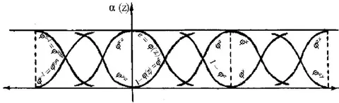
The analysis of monotone curves in Fig. 11 gives us only six varieties of the survival function as a function of density-dependent factors relative to some fixed value of $d^{\prime }(d^{\prime }\in {\mathbf{Z}}^{+}-\text{the set of positive integers})$ (Fig. 12), and two varieties of the survival function as a function of density-independent factors relative to some fixed value of $l^{\prime }(l^{\prime }\in \mathbf{R})$ (Fig. 13).

{"image_source":{"path":"images/36c0be67d9ac58c26763fc292676ca4cdf8405604d50827bf1547008fb5fad41.jpg"},"content":"","chart_caption":[],"chart_footnote":[]} {"image_source":{"path":"images/3ef27c371735d8db613c06f704fbe57a139460b396c5c497d8c2d5a0d6a8f315.jpg"},"content":"","chart_caption":[{"type":"text","content":"Rice. 12: Six Varieties of the Survival Function as a Function of Density-Dependent Factors"},{"type":"text","content":"Fig. 13: Two Types of Survival Function as a Function of Density-Independent Factors"}],"chart_footnote":[]}

Of the six possible curves of the survival function as a function of density-dependent factors, two (Fig. 12, V and VI) completely coincide in shape with two types of curves of the survival function as a function of density-independent factors (Fig. 13, I and II).

3.3. Intersection in n -dimensional space

Let the volume formed by the intersection of the corresponding cylinders in n-dimensional hyperspace be given:

The intersection of these cylinders in a given hyperspace is given as follow:

In general, such intersections can be infinite in ${}^n$ the -dimensional hyperspace belonging to the set of monotone curves

If $K\times G$ a group acting on a set of monotone curves M, we denote it by T ( $K\times G=T$ ), then on the set M ${}^n$ the group will act

Using the results of the group-theoretical study of the population survival function and the above, we can write that for any two intersections $\bigcap _{i=1}^n{H}_i$ and $\bigcap _{j=1}^n{H}_j$ from $M^n\mathrm{\exists }t\in T^n$ is such that

Since the group $T^n$ acts on the set $M^n$ transitively, the elements of the set $M^n$ (different intersections) are symmetrical relative to each other with respect to the action of the elements of the group $T^n$.

An ecological niche can be considered as an intersection of volumes such as (17) in n-dimensional $H=\bigcap ^n{H}_i$.

hyperspace, i.e. as a certain n-dimensional hypervolume of survival $\prod _{i=1}^n\left|{\mathbf{M}}_i^n\right|$. From the assumption and relation (20) it follows that the various intersections (18) in the set $M^n$ are symmetrical relative to each other. This means that the survival hypervolumes of different species are symmetrical relative to each other. Moreover, this conclusion may be supported by another piece of evidence of pulsating niches.

3.4. On the Symmetry of the Survival Rate Function

This section deals with the symmetric relationship of the survival functions to each other. At the same time, I would like to briefly dwell on the concept of symmetry, and what exactly we have when we study the symmetrical relationship of environmental factors among themselves.

The concept of symmetry in a popular form is covered in the works of G. Weyl (1968), L. Tarasov (1982), A. Migdal (1983, 1989), I. Shafransky (1985), A. Sonin (1987), R. Feynman (1987) and S. Petukhov (1988).

The famous mathematician G. Weyl (1968) suggested a wonderful definition of symmetry, according to which an object is called symmetrical if it can be changed in some way, resulting in the same thing you started with. It is in this sense that we speak of the symmetry of the laws of physics. This means that physical laws or the ways of representing them can be changed in such a way that this does not affect their consequences (Weyl, 1968; Feynman, 1987). Symmetry is understood in this sense in this work.

Those operations of change, the consequences of the impact of which are not reflected in the nature of physical or biological laws, constitute the essence of the concept of symmetry (Alekseev, 1978; Achurkin, 1978).

The principles of symmetry (invariance) are divided into geometric and dynamic. In this case, geometric symmetry is the symmetry that can be directly seen (rotations in space, shifts in time, translation). Unlike geometric principles, dynamic principles of symmetry are formulated in terms of the laws of nature and relate to certain types of interactions rather than to any correlations between events. An example of dynamic symmetry can be group-theoretical transformations. In confirmation of this, we will cite what Sonin (1987) said: "Thus, in classical mechanics, symmetry has lost its visual geometric meaning. Now it appears in an abstract form as a condition under which the control describing this or that physical law does not change its form. In this case, the conditions themselves must form a group in the mathematical sense."

From the above it follows that the study of symmetry is the conduct of classification in the corresponding field of research. For this purpose, we conducted a group-theoretical study of the survival function. For this purpose, the behavior of the survival function of the species shown in Fig. 10a was chosen. $\alpha (z)=e$

By performing the following operations on these curves: shift (translation), rotation $\pi$ around the axis (perpendicular to the Z axis) and transformations $1-\alpha (z)$ the appropriate number of times, we can obtain all kinds of survival functions (Fig. 10). Group-theoretical study of these operations showed that they form a group (see 14 - 16 formulas). Moreover, the group $K\times G$ found acts on the set M (the set of all possible functions of survival rates) transitively, i.e. for any $\phi$ and $\psi$ from M $\mathrm{\exists }g\in K\times G$ such a thing that ${\phi }^g=\psi$. It follows from this that the various survival functions (M) considered by us (see Fig. 1, 2 and 10) relative to the action of the elements of the group $K\times G$ are in a symmetrical relationship with each other, i.e. any element of the set M can be obtained from any other element of the set M using the corresponding symmetry operation from the group $K\times G$. A clear example is shown in Fig.

From the above it follows that, knowing the survival function for one type of environmental factor, we can obtain survival functions for other environmental factors using the elements of the transformation group $K\times G$, i.e. group $K\times G$ plays the role of the law of transformation of the survival function of environmental factors. Moreover, this law of transformation operates regardless of the type of factors.

The symmetry of the survival function also indicates that all environmental factors: abiotic, biotic and anthropogenic, with respect to their survival functions, are closely related, i.e. different manifestations of the same function (Gulamov, Fayziev, 1992). This also speaks of the internal consistency of environmental factors among themselves.

The logical conclusion about the symmetry of various intersections of the survival function in n the -dimensional hyperspace, i.e. about the symmetry of the hypervolumes of species survival, is fully justified. This conclusion indicates the symmetry of ecological niches of different species.

3.5. About some of the group's ideas G

In the work of Gulamov and Fayziev (1992) and in other previously published works of ours (Gulamov, 1989, 1994, 2012 (a); Gulamov and Fayziev, 1990), the different nature of the survival function and their transformations were studied. Research has shown that all varieties of the survival function are essentially different modifications of the function:

where k is the steepness coefficient ( $k\in R$ ) and $z(t)$ is the value of any environmental factor (Z) at a given time $t(z(t)\in \mathbf{Z})$.

Knowing one law of change of the survival function (21), it is possible to derive any other using the appropriate transformation from the group G. The abstract nature of the group structure does not allow for transformations for applied purposes. In this regard, a problem arises: the need to study various G representations of the group G that would allow this theoretical premise to be applied in solving applied problems.

First, about the structure, nature and morphisms - objects to the study of which any group-theoretical research is ultimately reduced. The group $G$ in terms of forming and defining relations has the following form (Gulamov, Fayziev, 1992; Gulamov, 1994):

Studies of the behavior of the elements of the group G have shown that each of the generators of the group (4.9) forms a cyclic subgroup:

Let us consider a subset of the set of elements of a group $H$ of the following form: $C=\{x^{2n+1}{y}^{-(2n+1)},x^{-(2n+1)}{y}^{2n+1}\}$, where $n\in {\mathbf{Z}}^{+}$, $x=f(z-z^{\prime })$, $y=1-f(z-z^{\prime })$ (Gulamov, Fayziev, 1992; Gulamov, Khoshimov, 1997). Research shows that $\mathrm{\forall }n\in {\mathbf{Z}}^{+}$

Moreover, a subgroup $c$ of a group $G$ is its center, i.e. $c=Z(G)$ From the above it follows that:

Taking into account the properties of the element, c group G (22) can be rewritten as:

$\{x^n,a{x}^n\}$, where is $Z_2$ the type of the group $C$ and $D$, $Z=\{x^n|n\in \mathbf{Z}\}$ $\Rightarrow H/C\cong Z$, $G/C=D\times H/C$.

Analysis of the structure (23) shows that, firstly, the group $G_M$ is structurally much simpler than the group G, and secondly, $G\cong G_M$. This allows us to further study the group $G_M$ instead of G.

With respect to the generating elements of group $G_M$ (23), we assume: let be x a parallel transfer $(P)$; a be a symmetric transformation $(S_1)$ with respect to the perpendicular axis passing through the points $z^{\ast }$ of the abscissa axis; c be a symmetric transformation $(S_2)$ with respect to the horizontal (parallel to the abscissa axis) line passing through the middle of the interval [0,1] of the ordinate axis. In other words x-P, $a-S_1$, $c-S_2$.

Now let us consider transformations in a more general form - this transformation on the projective plane is defined in the following form:

The matrix of such a transformation has the form:

Let the elements of this transformation matrix satisfy the conditions: $a_{11}=1,a_{12}=0,a_{13}=z^{\ast },a_{21}=0,a_{22}=1,a_{23}=0,a_{31}=0,a_{32}=0,a_{33}=1$. Then we obtain the matrix of parallel translation along the axis z. Such a matrix has the form:

The entry $a_{13}=z^{\ast }$ means that the origin of coordinates is shifted to a point $z^{\ast }$ along the abscissa axis. Symmetric transformations $S_1$ for $S_2$ matrix (25) have the form:

Here the matrices $S_1,S_2,P$ are the essence of the elements a, c, x in the group $G_M$ (23), respectively. Research has shown that matrices form a group with the usual matrix multiplication operation. Let us designate this group as follows: $S_1,S_2,P$

Elements of the group $SM(3,R)$ satisfy all the properties of the group $G_M:S_1^2=S_2^2=E$, $S_1{S}_2=S_2{S}_1$, $P{S}_2=S_{2}P$, $S_{1}P{S}_1=P^{-1}$ And $P{S}_{1}P=S_1$. It follows from this that The obtained results allow us to write: $G\cong G_M\Rightarrow G\cong SM(3,R)$. This result satisfies the above statement of the problem $k\ge 1$. The following material is presented under the assumption that in (21). For this purpose, we rewrite equation (21) taking into account the coefficients of the transformation matrix (25) as follows: $G_M\cong SM(3,R)$.

Thus, the survival functions can be transformed depending on the impact of the group elements $SM(3,R)$ as follows:

The superscripts of these survival functions denote the effects of the group elements $SM(3,R)$ on the function of the type (21) according to the law (28). Such impacts transform the survival functions into appropriate forms – what needed to be solved (Gulamov, Khoshimov, 1997).

Depending on the value of the survival function in the optimal intervals for the corresponding environmental factors, one or another type of survival function curve can be selected, for example:

1. For the optimal interval $[z_1^{\ast },z_2^{\ast }]$, where $\alpha (z)=1$ corresponds to $S_{1}P$ and P the transformation.

2. For the optimal interval $[z_1^{\ast },z_2^{\ast }]$, where $\alpha (z)=0$ corresponds to $S_{1}P{S}_2$ and $P{S}_2$ the transformation.

3. For the origin of coordinates, where the $\alpha (z)=1$ transformation $S_1$ corresponds $E$.

4. For the origin of coordinates, where the $\alpha (z)=0$ transformation $S_2$ corresponds $S_1{S}_2$.

In this fourth point, the indicated transformations are sufficient to calculate the value of the survival function for all environmental factors of any type.

To summarize the above, it can be stated that in a group $SM(3,R)$ there will always be a transformation that allows us to move from one type of survival function to another according to the ecological factors of interest to us, which do not require preliminary research on this factor.

IV. ON THE SET OF INFORMATION MODELS

This section is devoted to a qualitative study of the nature of information models and their set DIMIFN (All possible mentally permissible diversity of information models of objects of the ideal and physical nature) (Gulamov, 2017; 2018; 2021 a).

It should be noted that the concepts of information and information models are associated with fundamental issues of deep concepts of natural and humanitarian sciences (Shileiko A., Shileiko T., (1983).

We begin our study of this issue with an analysis of scientific and technical publications that currently exist (Internet materials: ru.wikipedia.org; wiki. vspu. ru > users/wodolazov/model/index; best - exam. ru > znakovie - modeli /).

1. An information model (in a broad, general scientific sense) is a set of information characterized by the essential properties and state of an object, process, phenomenon, as well as its relationship with the outside world.

2. Information models cannot be felt or visualized; they have no material embodiment because they are built only on information. Information models are models created in a formal language (i.e. scientific, professional or specialized). Examples of formal models are all types of formulas, tables, graphs, maps, diagrams, etc. The information model is thus - a general scientific concept meaning both an ideal and a physical object of analysis.

3. The verbal information model is obtained as a result of human mental activity and is presented in verbal form; it is symbolic, i.e. it can be expressed in drawings, diagrams, graphs, formulas, etc.

In modern scientific research, the term "information model" is used for various scientific concepts, such as: the structure of an atom, DNA, quark, gluon, the chemical structure of hydrogen, circle, plane, n-dimensional space, Higgs field, electric field, etc. All this can be generalized under the term information model. And the set of information models (DIMIFN) can be represented as a forming and reflecting space-time continuum (Gulamov, 2018).

"Information" is the essence of physical or abstract quantities, it is a more general concept relative to the term "information model" (Shileiko A, Shileiko T., (1983). An information model is any logical, structured, informational-semantic, abstract expression (Gulamov, 2017; 2018).

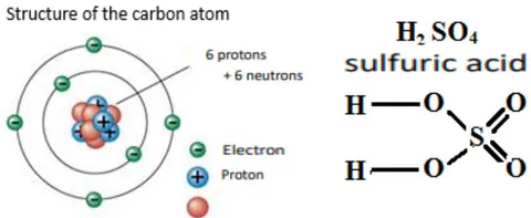
Examples of information models: mathematical expressions, functions and formulas:

physical and chemical structures (http://images.myshared.ru/4/319832/slide_1.jpg):

In the first and second chapters of this monograph, where the issues of interaction of environmental factors and the theoretical-group relationship of the function of survival rates were considered, the set of functions of survival rates (M) ( $\mathrm{\forall }i\alpha (A_i,t):\mathbf{R}\to [0,1]$, $i=1,2,\dots$ ), which is, in turn, an information model reflecting the interaction of an environmental factor on a biological object (Fig. 14).

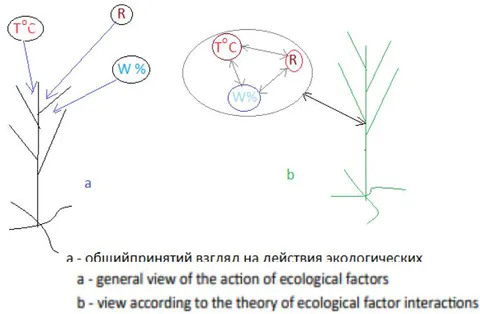
It would also be possible to cite many examples from the fields of biology and astronomy to information models, but within the framework of this work we will limit ourselves to references to Internet materials (berl.ru/article/kletka/dnk/..; medicalplanet.su/genetica/27. html; collectedpapers.com. ua/ru /...;). In a word, information models are any mathematical, physical, chemical, biological formalisms that have a hidden structure and dynamics that manifest themselves in the space-time continuum (Gulamov, 2018) and in theoretically conceivable ideal objects (mathematical formalisms and objects of a spiritual nature).

Information models have different kinds of variants. In mathematics, physics and chemistry, the same object can be represented by different information models in the form of a mathematical formula, graph, table or diagram. A more concrete and illustrative example can be given from biology: the number of genes in plant and animal species is in the thousands, each of which, through mutations, can produce dozens of alleles. Let us consider a simplified situation of the code in a haploid set, where there are only 1000 genes, each of which is capable of producing only 10 alleles through mutations. In this case, the number of gene combinations reaches ${10}^{1000}$ (each combination is an independent information model), that is, it reaches a huge value, which is greater than the number of electrons and protons in the Universe. If we translate all this into real species existing in nature and try to imagine the possible number of gene combinations, we will get infinity to the highest degree! This is the real unimaginable power of nature's biodiversity (Gulamov, 2016).

If we try to imagine various options of all possible conceivable and inconceivable mathematical, physical, chemical and biological information models, then we can definitely say that the set DIMIFN forms a set of infinite order of the power of the continuum.

In a word, the elements of the DIMIFN set are all possible variants of reflection of objects of the space-time continuum and abstract theoretical representations of their interaction. From the above it follows that there are two types of information models:

a) information models of objects of the physical world;

b) information models of an abstract (ideal) nature.

Item a) includes mathematical, physical, chemical, and biological descriptions of various natural phenomena and objects, for example: the phenomena of electricity, magnetism, gravity, elementary particles, and others. Item b) includes mathematical objects: arithmetic, algebraic, geometric operations, functions and the Holy Scriptures.

The nature of information models of any objects of the physical world is an immaterial entity that contains the information laws of the existence of physical objects. The nature of information models, regardless of the real existing natural objects, is given. Therefore, information models do not disappear, are not destroyed, are not lost, i.e. they are outside of space-time. An information model is like an immaterial beginning of the life of physical objects or a kind of hidden treasure of the physical world.

Information models are knowledge about physical and abstract (ideal) objects, processes and phenomena. If this assumption is taken as a basis, then with a high probability it can be said that any mathematical operations are specified in DIMIFN.

An information model, unlike information, only makes sense to humans. Any new knowledge can be obtained on the basis of operating with elements of the DIMIFN set. It is appropriate here to quote from the work of A. Shileiko, T. Shileiko (1983): "They say that I. Newton was once asked how he managed to discover the law of universal gravitation. "I thought about it!" was the answer." This means that I. Newton operated with the corresponding information models and eventually discovered a new information model – the law of universal gravitation!

The elements $(M_i,\text{rde }i\in N-\text{sets of natural numbers})$ of the DIMIFN set are not interconnected, but at the same time they can have the ability to combine with each other and with themselves in any quantity, thereby creating new information models of physical and ideal objects. In this case, an important condition for the combination is reasonable mutual correspondence. For example, the elements of the periodic table: they can be found in nature independently or in combinations in the form of some chemical or biological molecule.

The term "combinations" refers to certain structured mathematical, physical, chemical and biological formalisms.

Let us try to carry out some formalization of the set DIMIFN, taking into account some natural scientific generalizations:

1. The invariant nature of physical laws.

2. Transitions from a particular case to a general one and vice versa.

3. Elements of the periodic table and all kinds of chemical descriptions of physical and biological substances.

4. Genetic structures and descriptions of living objects, etc.

Considering the abstract nature of the elements of the infinite-dimensional set DIMIFN of the continuum cardinality, it is possible to carry out generalized algebraic formalization of the set DIMIFN (Gulamov, 2018):

each element of this set is a subset, that is,

$M_i=\{m_1,...,m_i,m_{i+1},...\}$, where $m_i\cap m_k\ne \mathrm{\varnothing }$, $i,k\in N$, (there is a combination between the elements of the subset $M_i$ ). The elements of the set DIMIFN ( $M_i$ ) can be of different dimensions $l(l=\overline{1,n})$. Naturally, the elements of the set DIMIFN, interacting with each other, can generate new all sorts of different elements: $M_i\cap M_j\ne \mathrm{\varnothing }$, perhaps, there are such elements of DIMIFN that do not interact: $M_r\cap M_k=\mathrm{\varnothing }$ (there is no combination between the elements).

Considering that the DIMIFN sets include all sorts of scientific and technical and abstract (ideal) sets and are to a high degree a superset, we can assume with high probability:

a) that there are subsets of the set DIMIFN $(M_i,M_j)$, where $Mor(M_i,M_j)$ and are given $Mor(m_i,m_j)$ (Fig. 16):

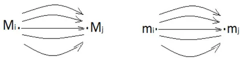
Rice. 16: All possible morphisms are a subset of the set DIMIFN $(M_i,M_j)$.

b) in many cases for DIMIFN elements $(M_i,M_j{M}_k)$ and the elements of its subsets $(m_i,m_j{m}_k)$ satisfy the law of composition (Fig. 17):

Fig. 17: Schematic reflections of the composition of DIMIFN elements $(M_i,M_j,M_k)$.

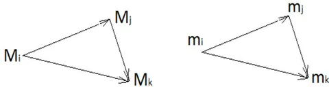
From the theory of interaction of environmental factors it follows that many elements of $(M_i,M_{i+1},\dots )$ the DIMIFN set are symmetrical with respect to the corresponding transformations (Gulamov, Krasnov, 2009; Gulamov, 2012 (b)).

All kinds of combinations and permutations of information models reflect new phenomena of the physical or ideal world that were previously unknown.

It is undeniable that the diversity of elements of the DIMIFN set is of an unimaginably high order.

4.1 On Generalized Set Operations Information Models

This section is a continuation of our previous works and is devoted to a qualitative study of the nature of the execution of generalized operations on elements of a set of all kinds of information models, mentally admissible for the diversity of objects of ideal and physical nature DIMIFN (All possible mentally permissible diversity of information models of objects of the ideal and physical nature) (Gulamov, 2017; 2018; 2020). For convenience, in the future we will simply call the DIMIFN set the set of information models (MIM).

The nature of the terms "information", "information model" and partially "set of information models" was analyzed in our previous works (Gulamov, 2018; 2020). In this paper, the execution of generalized operations on MIM elements will be formally described, to the extent possible, with appropriate examples. If we represent a set of information models (Gulamov, 2020):

then each element of this set represents a certain information model (IM). In turn, each IM consists of a certain number of information components (IK). It follows that each MIM element is a subset consisting of the corresponding information components, that is:

Depending on the level of complexity of the phenomenon being described, the number $I{K}_n^i$ in each $I{M}_i$ may be different.

Let us consider generalized operations: combinations, differentiations and recompositions over MIM elements. The generality of the operation of combination, differentiation and recomposition lies in the fact that they can be represented in the form of any mathematical operations or their combination, taking into account the observance of the principle of logical-constructive and logical-informational correspondence. The meaning of the terms of the operations we consider in this work is understood as follows:

A combination is a collection of parts together, one alongside the others in some kind of unity, coherence.

To differentiate means to dismember, to distinguish the separate from the particular when considering the whole.

Reassembly is the creation of a whole from many parts in a new way, relative to the original form.

MIM elements produces a specific type of information model. Differentiation of the corresponding elements of the MIM set generates a limited number of information components. By rearranging the results of the differentiation operation, it is possible to obtain a limited number of information models. These three operations are the basis of any research, knowledge, analysis and synthesis in the process of studying the environment. The degree to which the simulation models we have identified are reflected in reality depends on the successful application of the operations of combination, differentiation and recomposition. An instructive example is the hero of Arthur Conan Doyle's stories (1986), namely the actions of Sherlock Holmes, where he, by combining, differentiating, and recombining the collected information, is able to create the integrity of the completed event (a new information model).

I. Combinations: the action of this operation is that, by combining a certain number of elements MIM in logical-constructive and logical-informational correspondence, it is revealed $I{M}_r\in MIM$. The result may be previously known to us or new to us IM

The property of the combination operation in (1):

1. $\mathrm{\exists }I{M}_{i+r},I{M}_{k+l}\in MIM:I{M}_{i+r}\ast I{M}_{k+l}\ne \mathrm{\varnothing },$ information models $I{M}_{i+r},I{M}_{k+l}$ are combined in a logical-constructive combination.

2. $\mathrm{\exists }I{M}_{j+r},I{M}_{h+l}\in MIM:I{M}_{j+r}\ast I{M}_{h+l}=\mathrm{\varnothing }$, information models $I{M}_{j+r},I{M}_{h+l}$ are not combined in a logical-constructive combination.

3. $\mathrm{\exists }I{M}_i,I{M}_{i+r},I{M}_l\in MIM:(I{M}_i\ast I{M}_{i+r})\ast I{M}_l=I{M}_i\ast (I{M}_{i+r}\ast I{M}_l)=I{M}_n\in MIM$, the combination is associative.

4. $\mathrm{\exists }I{M}_l,I{M}_{l+r},I{M}_k\in MIM:(I{M}_l\ast I{M}_{l+r})\ast I{M}_k\ne I{M}_l\ast (I{M}_{l+r}\ast I{M}_k),$ the combination is not associative.

5. $\mathrm{\exists }I{M}_i,I{M}_{i+r}\in MIM:I{M}_i\ast I{M}_{i+r}=I{M}_{i+r}\ast I{M}_i=I{M}_j\in MIM$, the combination is commutative.

6. $\mathrm{\exists }I{M}_t,I{M}_{t+r}\in MIM$: $I{M}_t\ast I{M}_{t+r}\ne I{M}_{t+r}\ast I{M}_t$, the combination is not commutative.

Examples of the Combination Operation: Information models can be combined or not combined depending on the principle of their logical-constructive and logical-informational correspondence. More illustrative examples of compatible and incompatible things IM can be given from the fields of mathematics, physics, chemistry and biology. IM functions of the form $x^2+1=0$ and Newton's second law (F = ma) are not compatible because these two IM are not in logical-constructive and logical-informational correspondence. kxHooke's law (reflecting the action of elastic forces on a metal ball), the second (F = ma) and third laws (F = -F) of Newton are compatible IM. IMThe result of such a combination is a type $m\ddot{x}=-kx$ -a mathematical model of elastic vibrations of a metal ball. IM, characterizing the combination of chemical elements: sodium $1123N{a}_2{)}_8$ $1S^2,2S^2,2p^6,3S^1$ and chlorine $1735C{l}_2{)}_8$ $1S^2,2S^2,2p^6,3S^2,3p^5$ combine, and this combination is commutative. The result of this combination is NaCl. $24H{e}_{2}1S^2$ Helium and neon $1020N{e}_2{)}_{8}1S^2,2S^2,2p^6$ are incompatible according to the principle of logical-constructive and logical-informational correspondence. In the language of chemistry, this is explained as the completeness of the outer electron shells of the elements helium and neon. One can give many examples from the field of biology and ecology to the above-described properties of the combination operation, but the examples given quite convincingly reflect the idea.

II. Differentiation: the action of this operation is that most elements of MIM can be divided into a limited number of information components $(I{K}_n)$. There are some MIM elements that cannot be differentiated because they are not divided into information components, that is, they are considered a single whole IM. Fundamental world constants (physical, mathematical: the speed of light, Planck's constant, Boltzmann's,..., $\pi ...$ ) just relate to non-differentiable elements MIM. Non-differentiable elements of MIM are by their nature more compatible with other elements of MIM, thus they participate in the identification of new information models previously unknown to us.

Property of the Differentiation Operation in (1):

1. $\mathrm{\exists }I{M}_i\in MIM:I{M}_i=\{I{K}_1,I{K}_2,...,I{K}_n\},I{M}_i-differentiable$

1. $\mathrm{\exists }I{M}_k\in MIM:I{M}_k\ne \{I{K}_1,I{K}_2,...,I{K}_m\},I{M}_k-non-differentiable,thatis,itconsistsofasingle$ information – component $I{M}_k$.

Examples of the operation of differentiability. Differentiation of chemical structures of elements of the periodic table into electrons, protons and neutrons; differentiation of the ecosystem into ecological components; differentiation of DNA and RNA into nucleic acid sequences, etc.

III. Re-Arrangement: The effect of the recomposition operation is that the result of the differentiation operation $I{M}_i=\{I{K}_1,I{K}_2,...,I{K}_n\}$ can be recomposed in such a way that it can generate other IM, different from the original form $I{M}_i$. Various rearrangements and different information models are possible.

Properties of the Reflow Operation (1):

Let be $\{I{K}_1,I{K}_2,...,I{K}_n\}$ a set of information components. Different rearrangements of this set of information components can produce a variety of information models. As a result, it is possible to obtain the same or new, previously unknown ones IM. $\{I{K}_1,I{K}_2,...,I{K}_n\}$ There are also options where this differentiation is not recomposed in any other way than its original form.

Examples of the Recomposition Operation: Let us be given the information components: S -distance, t - time to travel this distance S, and v - speed to travel this distance. Various logical-constructive and logical-informational correspondences of these information components $(S,t,v)$ give us different information models: $S=v\cdot t$; $t=S/v$ and $v=S/t$. IMThus, we got different distances, times and speeds. All kinds of nucleic acid sequences can give rise to different DNA and RNA. Here all possible sequences correspond to a variety of combinations.

These operations are the basis of a generalized algorithm for cognition, research, analysis and synthesis of environmental studies and artificial intelligence.

IM that we are considering is not limited; they can be applied as much as necessary. The optimal execution of the above operations should be based on the principle of logical-constructive and logical-informational correspondence, that is, spatio-temporal correspondence to the imaginary reality. The above operations are the mechanism that generates all kinds of information models.

The operations of combination, differentiation and recomposition are the basis of any cognitive, scientific research and gaming processes, in other words, the basis of any intellectual processes. In these processes, the order in which the named operations are performed does not matter. The sequence of execution depends on the nature of the problem being studied, the relevant moment in time and location.

The object of research and study of human intelligence is information models of the surrounding world. The process of exploration and study of the world around humanity is not limited in the past, present or future. Therefore, the power of MIM is potentially infinite.

MIM elements do not impose any restrictions on MIM; on the contrary, they provide it with an infinite variety of continuum power. In a word, the MIM set is a universal set of all information models.

The set of survival rate functions with respect to the operations of superposition (translation (shift), rotation $\pi$ and transformation $1-\alpha (z)$ ), multiplicativity, and taking a minimum does not form an algebraic structure of a ring. Our analysis, taking into account the above-mentioned operations on the subject of the algebraic structure of the ring, showed that in MIM, firstly, it does not fulfill commutativity and, secondly, there is no inverse element.

V. ECOLOGICAL FIELD OF SURVIVAL

Before moving on to the concept of the "ecological field of survival" it is advisable to briefly explain the meaning of the term "physical field". In the work of V.I. Smirnova (1974) defines a physical field: "If some physical quantity has a certain value at each point in space or part of space, then the field of this quantity is determined in this way. If a given quantity is a scalar (temperature, pressure, electric potential), then the field is called scalar. If a given quantity is a vector (speed, force), then the field determined by it is called a vector field." Ya. B. Zeldovich and M. Yu. Khlopov (1988) explain this same term as follows: "Let a certain quantity be defined in space. This means that we can say what this quantity is at each point in space. For example, we know what the temperature is in a particular place. In this case, they say that the field of this value is given. In our example, it is a temperature field. If a rectangular coordinate system X, Y, Z is introduced into space, so that each point in space is characterized by the values of its coordinates, then the field is a function of the coordinates of each point and formally represents a function of three variables x,y,z. If the quantity whose field we are considering changes over time, then the field of this quantity depends on time and is called non-stationary. If a quantity does not depend on time, its field depends only on spatial coordinates and is called stationary" (Zeldovich, Khlopov, 1988).

Currently, there are various names for physical fields: gravitational, electromagnetic, strong and weak nuclear, quantum and Higgs fields. More detailed information about physical fields is given in Internet materials (https://ru.wikipedia.org > wiki > 2021).

To reveal the concept of "ecological field of survival", we need to reveal such concepts as ecological factor, survival function, habitat (Gulamov, 1982; 1994; 1997; 2012 (a); Gulamov, Logofet, 1997).

An environmental factor is a certain physical and/or biological force that changes according to certain patterns $f(A_i)$ and manifests itself as a condition or element of the environment $A_i$, which is capable of directly or indirectly influencing a living organism, at least at one stage of its individual development (Gulamov, 1982; 2012 (b)):

Environmental factors interact with biological objects, and biological objects respond with adaptive reactions, acting as biological factors, and this, in turn, gives grounds to speak about the interaction of environmental factors.

In nature, environmental factors affect biological objects in a complex manner. The nature and significance of the complex impact depends on the nature of the interaction of environmental factors with each other.

When environmental factors interact, a certain state always arises, which is called the environment. If we assume that the environment is a formative and determining process, then it becomes clear that environmental factors act on biological objects simultaneously and jointly, that is, in a complex manner.

Adaptive reactions of biological objects to the impact of environmental factors is the survival of these objects. If the specific adaptive response of biological objects is understood as their survival, then we can talk about the maximum or minimum survival of biological objects in connection with the impact of environmental factors. It follows that for each environmental factor there are certain intervals of optimality where the survival rate of biological objects is maximum. Survival is the ability of an organism or population to withstand the impact of an environmental factor. The impact of environmental factors on individuals of a population should be taken into account through the concept of the survival function. We represent the survival function as a quantitative expression of the survival of organisms or individuals of a population, which characterizes the impact of an environmental factor and is a scalar value. The survival function can be chosen as a monotone function mapping R (sets of real numbers) onto a segment $[0,1]$ using the example of an environmental factor $A_i$:

In reality, the survival of an organism or individuals of a population at any given moment in time tis determined by the influence of a complex of factors:

Where $N(t)$ and $N(t+1)$ – the number of individuals in the population at time t and $t+1$ respectively.

Each biological species differs from each other in its characteristic ecological value – the values of the survival function, $\left(\alpha (\overrightarrow{A},t)\right)$ respectively. It follows that each point of the survival space (habitat) at each moment in time $(x,y,z,t)$ is characterized by a set of values of the survival function of the corresponding biological species:

Where $(x,y,z,t)$ – coordinate of the survival space at the corresponding moments of time, $\{{\alpha }_1(\overrightarrow{A},t),{\alpha }_2(\overrightarrow{A},t),...,{\alpha }_m(\overrightarrow{A},t)\}$ – corresponding values of the survival function m of biological species. Since biological species are different, it is natural that the values of their survival function differ from each other.

Against the background of the above definitions and examples of physical fields, we can say that the ecological value we have described – the survival function $(1,2)$ – determines the ecological field of survival of a population or biological species in the survival space (habitat). The ecological field of survival, by the nature of the survival function $(1)$, is a non-stationary scalar field (Gulamov, 2021(b)).

Depending on the type of combination of environmental factors and their quantity at different points in the survival space (habitat), the values of the survival function of individuals in the population will be different. If there are biological species min this survival space, then each point of the survival space under consideration is characterized by a different value m of the survival function pieces (3).

Each point of the ecological field of survival, unlike other physical fields, at each moment in time is characterized by a multiple value (3) of the survival function of the corresponding biological species, otherwise known as a multidimensional survival function (Gulamov, Terekhin, 2004).

The environment-forming ecological factors, the number of species of biodiversity and the presence of corresponding trophic chains at different points of the habitat vary over time, hence the "tension" (value m) (3) of the ecological field of survival, which is also changeable. All this points to the complex nature of the "pulsation" of the non-stationary scalar ecological field of survival.

The uneven distribution of biological species in the survival space (in the habitat) is explained by the variability of the structure of the ecological survival field (3).

VI. CONCLUSION

This monograph studies the issues of theoretical prerequisites of ecological algebra: basic aspects of the theory of interaction of ecological factors; group-theoretical relations of the survival rate function, information models, generalized operations over a set of information models and ecological survival fields. This was the first time that the problem was formulated in this way.

Summarizing the theoretical research on the above aspects in this monograph, the following conclusions can be drawn.

According to the theory of interaction of environmental factors:

Ecological factors: firstly, these are diverse (potentially unlimited) variable natural forces; secondly, the adaptive reactions of biological objects to the impact of ecological factors is their survival; thirdly, the impact of environmental factors on individuals of a population should be taken into account through the concept of the survival function; fourthly, despite the potentially infinite varieties of ecological factors, the functions of survival coefficients corresponding to them can be divided into six varieties.

The interaction of environmental factors is a certain hypervolume of survival, formed by the interaction of the function of survival coefficients of the corresponding environmental factors among themselves.

By replacing the term "set" in Hutchinson's definition of an ecological niche with a "fuzzy set", i.e. allowing non-binary well-being functions as indicator functions, in other words, replacing ecological factors with survival functions, we obtain a definition of a generalized, one might say, "fuzzy" ecological niche. This generalization seems to us as natural as the use of softer survival functions corresponding to them instead of ecological factors. It is obvious that blurred ecological niches can more adequately describe real situations.

Our group-theoretical studies of six varieties of the function of survival coefficients of ecological factors show that: firstly, all possible monotonic functions of survival coefficients (M) differ from each other only in the parameters of steepness and shift. And with respect to the translation operation (shift), rotation by $\pi$ and transformations $1-\alpha (z)$ form a non-Abelian infinite-dimensional group $K\times G$; secondly, the invariance of the form of the survival rate function is

the corresponding ecological factors indicates that all ecological factors – abiotic, biotic and anthropogenic – are closely related in relation to their functions of the survival coefficient, i.e. they constitute different manifestations of the same function. This indicates the internal consistency of environmental factors with each other, in other words, environmental factors are symmetrical relative to each other.

According to research on simulation models:

An information model is any logical, structured, informational-semantic, abstractly expressed physical or immaterial (ideal) object.

All kinds of combinations of information models generate a variety of conceivable or inconceivable information models of physical and ideal objects that have not been previously identified.

Knowledge of the nature of the physical and ideal world is based on the analysis and synthesis of their various information models and on the identification of corresponding new information models.

The set of survival coefficient functions is a simulation model of the survival of biological objects, and is therefore a subset of the sets of simulation models.

The set DIMIFN of the power of the continuum.

The set DIMIFN contains all kinds of mathematical operations: morphisms, homomorphisms, compositions, etc.

On the study of generalized operations on a set of simulation models (MIM):

Any information model is the result of applying the operations of combination, differentiation and recomposition. The order in which the above operations are performed does not matter. The main thing is to comply with the principle of logical-constructive and logical-informational correspondence.

The mechanism of any cognitive process is the operations of combination, differentiation and recomposition.

MIM is an open set with respect to the operation of combination, differentiation, and recomposition.

Non-differentiable elements MIM can be taken as IMan information component.

The implementation of variants of equally possible combinations and reconfigurations is dictated by dissipative, bifurcation, attractor, synergetic and other nonlinear states of the structure of spatio-temporal structures.

The subset of the survival rate function, the MIM set, with respect to superposition operations (translation (shift), rotation on $\pi$ and transformation $1-\alpha (z)$ ), multiplicativity and taking a minimum is an open subset.

According to research on the ecological field of survival:

The ecological value, a function of the survival rate of biological species in the environment, determines the non-stationary scalar ecological field of survival.

Each point of the ecological field of survival, unlike other physical fields known in science, is characterized by several values of the survival function.

Variability over time, environment-forming ecological factors, biodiversity and trophic chains form the "pulsating" nature of the non-stationary scalar ecological field of survival.

The reason for the heterogeneity of ecological systems is the variability of their biotic components over time, in other words, the "pulsating" nature of the ecological field of survival.

The fundamental basis of theoretical ecology is the study and research of the algebraic properties of ecological phenomena. One of the main ecological phenomena is the interaction of ecological factors and the formation of corresponding survival functions in biological objects for this interaction.

All the beauty in nature is when the human "voice" is in unison with the great "symphony" of nature.

INTERNET MATERIALS

About the Author: Gulamov Muhammad Isakovich Born: December 1, 1953

Currently serving as an independent researcher, I specialize in various aspects of ecological science and mathematical modelling. My primary research interests include the mathematical modelling of ecological factor interactions and ecological niches, the algebra of ecology, biodiversity theory, the biophysics of ecosystems, and the development of information models.

Academic Background:

• Candidate of Sciences Dissertation: Successfully defended on April 26, 1987, at the Doctoral Council on Biophysics, Institute of Biophysics, Siberian Branch of the Academy of Sciences of the USSR, Krasnoyarsk.

Dissertation Topic: "Simulation Model of the 'Parasite-Host' System: Wasp-Winter Cutworm (Cotton Pest)." Degree: Candidate of Physical and Mathematical Sciences.

• Doctoral Dissertation: Defended on December 19, 2001, at the Doctoral Council on Ecology, K.A. Timiryazev Moscow Agricultural Academy, Moscow. Dissertation Topic: "Modelling and Research of the Interaction of Ecological Factors." Degree: Doctor of Biological Sciences.

Publications and Contributions: I have published 83 scientific works, including 2 preprints, 6 monographs, 8 teaching aids, 2 textbooks, and 1 publication in Scopus. My most significant works have been featured in prestigious academic journals of the USSR Academy of Sciences, the Russian Academy of Sciences, Tajikistan, Uzbekistan, and reputable Western publications.

Professional Engagement:

• I played a key role in organizing major conferences on mathematical ecology within the CIS, notably in Dushanbe (1991) and Bukhara (1992).

• Collaborating with renowned specialists from leading Russian institutions, such as:

• Tver State University

• Tver Agricultural Academy

• Computing Center of the Russian Academy of Sciences (VTs RAN)

• Lomonosov Moscow State University (MSU)

• Laboratory of Mathematical Ecology, Institute of Atmospheric Physics, Russian Academy of Sciences

• Institute of Applied Mathematical Research, Russian Academy of Sciences (Petrozavodsk)