Does Super Kamiokande Observe L´evy Flights of Solar Neutrinos?

I. SOLAR NEUTRINOS: SUPERKAMIOKANDE DATA

Over the past 50 years, radio-chemical and real-time solar neutrino experiments have proven to be sensitive tools to test both astrophysical and elementary particle physics models and principles (Sakurai, 2018; Orebi Gann et al., 2021). Solar neutrino detectors (radio-chemical: Homestake, GALLEX + GNO, SAGE, real-time: SuperKamiokande, SNO, Borexino) have demonstrated that the Sun is powered by thermonuclear fusion reactions. Today fluxes, particularly from the pp-chain have been measured: pp. Be, pep, B, and, hep. Experiments with solar neutrinos and reactor anti-neutrinos (KamLAND) have confirmed that solar neutrinos undergo flavor oscillations (Mikheyev-Smirnov-Wolfenstein (MSW) model). Results from solar neutrino experiments are consistent with the Mikheyev-Smirnov-Wolfenstein Large Mixing Angle (MSW-LMA) model, which predicts a transition from vacuum-dominated to matter-enhanced oscillations, resulting in an energy dependent electron neutrino survival probability.

{"image_source":{"path":"images/d13baebb46e13e359b573352d30eb90f9505c889aed8a1cb17fa5a6ab8150f88.jpg"},"content":"","chart_caption":[{"type":"text","content":"Figure 1: Yearly solar neutrino flux measured by SuperKamiokande. The redfilled circle points show the SuperKamiokande data with statistical uncertainty and the gray striped area show the systematic uncertainty for each phase. The horizontal black solid line (red shaded area) shows the combined value of measured flux (its combined uncertainty). The black-blank circle points show the sunspot numbers from 1996 to 2018 (Abe et al., 2024)"}],"chart_footnote":[]}

II. DIFFUSION ENTROPY AND STANDARD DEVIATION: ANALYSIS

For all radio-chemical and real-time solar neutrino experiments, periodic variation in the detected solar neutrino fluxes have been reported, based mainly on Fourier and wavelet analysis methods (standard deviation analysis). Other attempts to analyze the same data sets, particularly undertaken by the experimental collaborations of real-time solar neutrino experiments themselves, have failed to find evidence for such variations of the solar neutrino flux over time (Abe et al., 2023). Periodicities in the solar neutrino fluxes, if confirmed, could provide evidence for new solar, nuclear, or neutrino physics beyond the commonly accepted physics of vacuum-dominated and matter-enhanced oscillations of massive neutrinos (MSW model) that is, after 50 years of solar neutrino experiment and theory, considered to be the ultimate solution to the solar neutrino problem (Figure 1).

{"image_source":{"path":"images/742a5960409c8b7cba8dc8321920eacf6255a21dd15f37f9435478cdc90bd488.jpg"},"content":"","chart_caption":[{"type":"text","content":"Figure 2: Measured "},{"type":"equation_inline","content":"{}^{8}B"},{"type":"text","content":" solar neutrino fluxes for 5-day (top five panels, black data points) and 45-day (bottom panel, blue data points) intervals without "},{"type":"equation_inline","content":"1/R^{2}"},{"type":"text","content":" correction. The errors in the 5-day (the 45-day) plot are asymmetric (symmetric) errors of the average fluxes. The solid-red curve in the 45-day plot is the expected sinusoidal solar neutrino flux based on the elliptical orbit of the Earth Abe et al., 2023."}],"chart_footnote":[]}

Specifically, subsequent to the analysis made by the SuperKamiokande collaboration, the SNO experiment collaboration has painstakingly searched for evidence of time variability at periods ranging from 10 years down to 10 minutes. SNO has found no indications for any time variability of the flux at any timescale, including in the frequency window in which -mode oscillations of the solar core might be expected to occur. Despite large efforts to utilize helio-seismology and helio-neutrinospectroscopy, at present time there is no conclusive evidence in terms of physics for time variability of the solar neutrino fluxes from any solar neutrino experiment. If such a variability over time would be discovered, a mechanism for a chronometer for solar variability could be proposed based on relations between properties of thermonuclear fusion and g-modes (Buldgen et al., 2024; Sturrock et al., 2021).

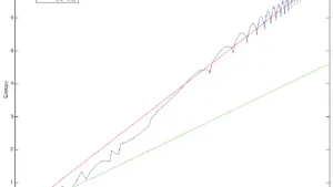
All above findings encouraged the conclusion that Fourier and wavelet analysis, which are based upon the analysis of the variance of the respective time series (standard deviation analysis: SDA) should be complemented by the utilization of diffusion entropy analysis (DEA), which measures the scaling of the probability density function (pdf) of the diffusion process generated by the time series thought of as the physical source of fluctuations (Scafetta, 2010). For this analysis, we have used the publicly available data of SuperKamiokande-I (1996-05-31 - 2001-07-15) and SuperKamiokande-II (2002-12-10 - 2005-10-06) (see Figure 2) (Yoo et al., 2003: Cravens et al., 2008; Abe et al., 2024). Such an analysis does not reveal periodic variations of the solar neutrino fluxes but shows how the pdf scaling exponent departs in the non-Gaussian case from the Hurst exponent. Figures 3 and 4 show the scaling exponents (DEA) for the SuperKamiokande I and II data. The respective Hurst exponents for SDA are visible in Figures 5 and 6 (Haubold and Mathai, 2018, 2025). SuperKamiokande is sensitive mostly to neutrinos from the and hep branch of the pp nuclear fusion chain in solar burning. Above approximately 4 MeV the detector can pick-out the scattering of solar neutrinos off atomic electrons which produces Cherenkov radiation in the detector. The and rarer hep neutrinos have a spectrum which ends near 20 MeV.

Assuming that the solar neutrino signal is governed by a probability density function with scaling given by the asymptotic time evolution of a pdf of x, obeying the property (Scafetta, 2010; Culbreth et al, 2023; Beghin et al. 2025)

where denotes the scaling exponent of the pdf. In the variance based methods, scaling is studied by direct evaluation of the time behavior of the variance of the diffusion process. If the variance scales, one would have

where is the variance of the diffusion process and where H is the Hurst exponent. To evaluate the Shannon entropy of the diffusion process at time t, defined as

and with the previous one has

The scaling exponent is the slope of the entropy against the logarithmic time scale. The slope is visible in Figures 3 and 4 for the SuperKamiokande data measured for and hep. The Hurst exponents (SDA) are H = 0.66 and H = 0.36 for and hep, respectively, see Figures 5 and 6 (Mathai and Haubold, 2018). The pdf scaling exponents (DEA) are and for and hep, respectively, as shown in Figures 3 and 4. The values for both SDA and DEA indicate a deviation from Gaussian behavior which would require that .

A test computation for the application of SDA and DEA to data that are known to exhibit non-Gaussian behavior have been published by Haubold et al. (2012) and Tsallis (2024). In this test computation, SDA and DEA, applied to the magnetic field strength fluctuations recorded by the Voyager-I spacecraft in the heliosphere clearly revealed the scaling behavior of such fluctuations as previously already discovered by non-extensive statistical mechanics considerations that lead to the determination of the non-extensivity q-triplet.

2.1 The Principle of Scaling Model

Let x be a real scalar random variable having the density . Then on the support of x, that is, whenever . Let a > 0 be a real scalar constant. Suppose that we wish to determine the density of the scaled x, namely ax. Let {"image_source":{"path":"images/471821ebe038c48582c3a10f008bebab6396756024a85004357d560d5c80e016.jpg"},"content":"","chart_caption":[{"type":"text","content":"Figure 3: The Difusion Entropy Analysis (DEA) of the "},{"type":"equation_inline","content":"{}^{8}B"},{"type":"text","content":" solar neutrino data from the SuperKamiokande I and II experiment."}],"chart_footnote":[]}

{"image_source":{"path":"images/afbe9724248bda9889e2c02bf0b4825a739b58fe13740d031903ea56822a3008.jpg"},"content":"","chart_caption":[],"chart_footnote":[]} {"image_source":{"path":"images/216c62ca4f4e2c0f4a5a94cf2130a19d59bd30c9b5d7679e4270f2587f5a622b.jpg"},"content":"","chart_caption":[{"type":"text","content":"Figure 4: The Difusion Entropy Analysis (DEA) of the hep solar neutrino data from the SuperKamiokande I and II experiment."},{"type":"text","content":"Figure 5: The Standard Deviation Analysis (SDA) of the "},{"type":"equation_inline","content":"{}^{8}B"},{"type":"text","content":" solar neutrino data from the SuperKamiokande I and II experiment."}],"chart_footnote":[]}

{"image_source":{"path":"images/2011c7bddaf02589cbc1d45cdbaa5612523aee03dd58555342584a3d39fa885c.jpg"},"content":"","chart_caption":[{"type":"text","content":"Figure 6: The Standard Deviation Analysis (SDA) of the hep solar neutrino data from the SuperKamiokande I and II experiment."}],"chart_footnote":[]}

where is a positive constant. Let be the density of . Then

What is the mean value and variance of the scaled ? Let denote the expected value or mean value of and let . Then,

which means that the mean value is scaled a and the variance is scaled by . Suppose that . Then, the mean value of x is scaled by and the variance is scaled by . What happens to Shannon entropy? Shannon entropy for a discrete distribution , denoted by , is given by

where c > 0 is a constant. This negative sign is taken because and hence, in order to make a minus sign is taken. The corresponding continuous case is the following:

Even though is the density of x, it need not remain less than one, still a minus sign is taken because the probability over the interval dx is which is always less than one, there by and such sums are there in the integral. Hence the notation corresponds to that in the discrete case . What happened to Shannon entropy in the scaled case? Note that in the scaled case the density of the scaled x, namely y = ax, is given by . Hence

This is the change where and are Shannon entropy on f and g respectively. If , then .

If the staring variable is a vector or a matrix X, then the scaling constant can be a real scalar quantity a > 0 or a real positive definite matrix A so that Y = aX or Y = AX will be the scaled model. When matrices are involved, we can have scaling matrices and so that we may take where B is another real positive definite matrix. In the case of matrices or sequence of matrices we can incorporate scaling in many different ways.

In a practical situation, usually the scaling constant a > 0 may have its own prior distribution. For example, if where if t is the time parameter then the behavior of may change for different t values or at different epochs of time, which means t has its own distribution.

2.2 Prior Distribution for the Scaling Parameter

Suppose that the scalar variable be positive and has a gamma density of the form

and elsewhere. Consider a scaled x, namely y = ax, a > 0. Then, the density of y, , is the following:

Suppose that and suppose that , then for the density of y is the following:

Suppose that and x has a Gaussian density

Then, has the density

Suppose that the scaling constant a has a prior density. In this case we may write g(y) as g(y|a) = density of y at a given a. If h(a) is a prior density for a, then the joint density of a and y is g(y|a)h(a) = \frac{1}{a}f(\frac{y}{a})h(a). Then the unconditional density of y or the density of y for all values of a, is given by the following and denoted by g_{y}(y):

Suppose that is the density

and zero elsewhere. Suppose that is Gaussian with . Then,

This is Bessel type integral which was evaluated earlier. This integral has the structure of the Mellin convolution of a product, namely

This is Bessel type integral which was evaluated earlier. This integral has the structure of the Mellin convolution of a product, namely

where

Then the Mellin transforms of and , denoted by , with the Mellin parameter , are the following:

Hence, for ,

This H-function, denoted by , is the following after writing :

By using the duplication formula for gamma functions, we can write

Then

When is not an odd positive integer, then the poles of the integrand are simple and one can evaluate the above G-function as a linear function of three hypergeometric functions by using residue calculus as illustrated below for one such series. Consider the poles of . They are at . Let the sum of the residues be denoted by . Then

But for

Then,

Hence,

III. PROBABILITY DENSITY FUNCTION AND DIFFERENTIAL EQUATION: LEVY FLIGHTS

We consider a diffusion process generated by a waiting time pdf with a finite characteristic time T that can be modeled with a Poissonian distribution, and a jump length pdf given by a Lévy distribution with index (Metzler and Klafter, 2000). The Fourier transform of is

Then has the asymptotic behavior given by

for and . Substituting the asymptotic expansion of the jump length pdf in the Fourier space and the waiting time pdf of

where is the characteristic waiting time in the Laplace space into

where is the Fourier transform of the initial condition , we obtain the following jump pdf in the Fourier-Laplace space

where is the generalized diffusion constant. Eq.(9) is the solution of the generalized diffusion equation (Hilfer, 2018)

where is the fractional Weyl operator. Upon Laplace inversion of Eq. (9), we get the characteristic function of the jump pdf

Eq.(11) is the characteristic function of a centered and symmetric Lévy distribution. The Fourier inversion of (7) can be analytically obtained by making use of the Fox function (Mathai et al., 2010; Mathai and Haubold, 2018)

, where c in the contour is such that . Replacing by s, observing that coming from s ds is canceled with sitting outside, we have the following:

By using the duplication formula for gamma functions, we have

so that one is canceled. Then,

Evaluating the H-function as the sum of the residues at the poles of , which are at , we have the following series:

IV. DISCUSSION

The first solar neutrino experiment led by Raymond Davis Jr. showed a deficit of neutrinos relative to the solar model prediction, referred to as the solar neutrino problem since the 1970s. The Kamiokande experiment led by Masatoshi Koshiba successfully observed solar neutrinos, as first reported in 1980s. The solar neutrino problem was solved due to neutrino oscillations by comparing the SuperKamiokande and Sudbury Neutrino Observatory results. While recent decades have offered tremendous advances in solar neutrinos across the fields of solar physics (Buldgen et al., 2024; Yang and Tian, 2024), nuclear physics (Bertulani et al., 2022; Hwang et al., 2023), and neutrino physics (Sturrock et al., 2021; Slad, 2024), many lingering mysteries remain.

This chapter takes advantage of publicly available solar neutrino SuperKamiokande data and analyses them by applying diffusion entropy analysis and standard deviation analysis. The result is a scaling exponent indicating anomalous diffusion of solar neutrinos in terms of Lévy flights. Based on this result the chapter develops the probability density function for neutrino flights and derives the respective differential equation in terms of a fractional Fokker-Planck equation. Accordingly, the closed form analytic representation of the neutrino power density function is given as a Fox H-function that can be used for further numerical exercises for the benefit of solar neutrino physics.