
Published On July 15, 2024
Journal Issue LJRS Volume 24 Issue 9

On Multiverses (or Parallel Universes) of Matrix Triple Solutions of the Diophantine Equation X3 + Y 6 = Z

Dr. Joachim Moussounda Mouanda
Article Fingerprint
Research ID 1HU41

IntelliPaper

Abstract

We show that the Diophantine equation X 3 + Y 6 = Z 6 (0.1) admits matrix triple solutions from M3(N) and M6k(N), k ∈ N. We construct infinite universes made of these solutions. We introduce different construction structures sets of matrix solutions associated to the Diophantine equation (0.1). These construction structures sets of matrix solutions allow us to show that there exists an infinite number of multiverses (parallel universes) of the matrix solutions of the Diophantine equation (0.1) containing each a finite number of universes of matrix triples.

Explore Digital Article Text

I. INTRODUCTION AND MAIN RESULT

A multiverse (or parallel universes) is the collection of alternate universes that share a universal hierarchy. The idea of the existence of the multiverse has been around for long time. An idea which many theoretical physicists have been trying to prove by using string theory which is a branch of theoretical physics that attempts to reconcile gravity and general relativity with quantum physics. In 2018, Stephen Hawking on his paper entitled "A smooth exit from eternal inflation?" predicted that there are not infinite parallel universes in the multiverse, but instead a limited number and these universes would have laws of physics like our own [4]. The idea of multiverse is not sufficiently understood to the most mathematicians. Perhaps the lack of understanding the existence of the multiverse is due to the fact that mathematicians never deeply study the idea of multiverse in terms of tuples of numbers satisfying an equation (E) which represents the universal stability law of universes contained in the multiverse. Generating universes of tuples of numbers (or matrices) which satisfy a certain equation (E) is an interesting approach. In 2021, Mouanda introduced a new method of computing the Galaxies of sequences of Pythagorean triples [5]. He constructed the multiverse of Pythagorean triples of complex numbers which has a finite number of universes since

\[\mathcal{F}_{2,2,2}(\mathbb{N}) \subset \mathcal{F}_{2,2,2}(\mathbb{Z}) \subset \mathcal{F}_{2,2,2}(\mathbb{Q}) \subset \mathcal{F}_{2,2,2}(\mathbb{R}) \subset \mathcal{F}_{2,2,2}(\mathbb{C}).\]

This lead to the introduction of the new theory called "Galaxies Number Theory". This new theory provides us a better understanding of the laws and structures of different universes. The study of the galaxies of the universe of Pythagorean triples of positive integers (matrices or polynomials) gives us a clear understanding of parallel universes. Pythagorean triples have been known and developed since ancient times with the oldest record dating back to 1900 BC [1]. Finding methods for generating Pythagorean triples have been of great interest to mathematicians since Babylonians (from 1900 to 1600 BC). In the literature, there are three classical methods of generating Pythagorean triples. Namely, Pythagoras' method (c. 540BC), Plato's Formula (c. 380 BC) [8] and Euclid's formula (c. 300BC) [2]. There are in three post-classical methods which are Fibonacci's method (c. 1170 - c. 1250), Stifel's method (1544) [11] and Ozanam's Method (1694)[9]. There are two modern methods which are Portia's method and Dickson's method [10, 3]. Recent Mouanda's work on finding the matrix solutions of Diophantine equations shows that matrix exponential Diophantine equations always admit an infinite number of matrix solutions [6].

In this paper, we show that the Diophantine equation admits not only matrix solutions from the set but also matrix solutions from the set . We give some examples of matrix solutions. We construct universes made of these solutions. We introduce different construction structures sets of matrix solutions associated to this Diophantine equation. These construction structures sets of matrix solutions allow us to construct the multiverses (parallel universes) of matrix triple solutions of the Diophantine equation containing each a finite number of universes.

Theorem 1.1. There exists an infinite number of multiverses (parallel universes) of matrix triple solutions of the Diophantine equation containing each a finite number of universes of matrix triples.

II. PROOF OF THE MAIN RESULT

In this section, we construct universes of matrix triple solutions of the Diophantine equation (0.1). We introduce the construction structures sets of matrix triple solutions of this equation. We construct the multiverses of matrix triple solutions of the equation (0.1).

2.1 The Universe of Matrix Triple Solutions of the Diophantine Equation

Let be a function of three variables. Define by

\[\mathcal {F} (\mathbb {N} ^ {3}) = \left\{(x, y, z): f (x, y, z) = 0 \right\}.\]

The set is called the universe of triples of positive integers. Every element of the set is called a planet. The equation is called the stability law of the universe .

Example 1: Let be a function of three variables such that

\[(x, y, z) \longmapsto f _ {n, m, k} (x, y, z) = x ^ {n} + y ^ {m} - z ^ {k}.\]

In this case,

\[\mathcal {F} _ {n, m, k} (\mathbb {N} ^ {3}) = \left\{(x, y, z) \in \mathbb {N} ^ {3}: f (x, y, z) = 0 \right\} = \left\{(x, y, z) \in \mathbb {N} ^ {3}: x ^ {n} + y ^ {m} = z ^ {k} \right\}.\]

Fermat's Last Theorem allows us to say that , with .

Example 2: The universe

\[\mathcal {F} _ {2, 2, 2} (\mathbb {N} ^ {3}) = \left\{(x, y, z) \in \mathbb {N} ^ {3}: x ^ {2} + y ^ {2} = z ^ {2} \right\}\]

has an infinite number of elements. The set is called the universe of Pythagorean triples.

Mouanda's recent work on finding matrix solutions of Diophantine equations shows that the universe

\[\mathcal{F}_{n,m,k}(M_{nmk}(\mathbb{N})^3) = \left\{(X,Y,Z) \in M_{nmk}(\mathbb{N})^3 : X^n + Y^m = Z^k\right\}\]

is not empty at all for every triple of positive integers. Assume that n=3 and m=k=6. Let us construct subsets of the universe

\[\mathcal{F}_{3,6,6}(M_6(\mathbb{N})^3) = \left\{(X,Y,Z) \in M_6(\mathbb{N})^3 : X^3 + Y^6 = Z^6\right\}\]

Definition 2.1. [7] A matrix is a construction structure of matrix solutions of Diophantine equations if there exist two positive integers such that .

Denote by

\[D_{n}(\mathbb{N}) = \left\{B \in M_{n}(\mathbb{N}): B^{m} - \beta \times I_{n} = 0, m, \beta \in \mathbb{N}\right\}\]

the set of all construction structures of matrix solutions of Diophantine equations from . A matrix Diophantine equation can admit several construction structures. Let be a positive integer. Let

\[A_{\alpha} = \left( \begin{array}{c c c c c c} 0 & 1 & 0 & 0 & 0 & 0 \\0 & 0 & 1 & 0 & 0 & 0 \\0 & 0 & 0 & 1 & 0 & 0 \\0 & 0 & 0 & 0 & 1 & 0 \\0 & 0 & 0 & 0 & 0 & 1 \\\alpha & 0 & 0 & 0 & 0 & 0 \end{array} \right)\]

be a Rare matrix of order 6 and index 1 [6]. The matrix allows us to construct an infinite number of matrix solutions of the Diophantine equation . Indeed, let us notice that . This implies that

\[\left\{ \begin{array}{l} A _ {\alpha} ^ {2 \times 3} = \alpha \times I _ {6} \\ A _ {\beta} ^ {6} = \beta \times I _ {6} \\ A _ {\alpha + \beta} ^ {6} = (\alpha + \beta) \times I _ {6} \\ (A _ {\alpha} ^ {2}) ^ {3} + A _ {\beta} ^ {6} = (\alpha + \beta) \times I _ {6} = A _ {\alpha + \beta} ^ {6}, \forall \alpha , \beta \in \mathbb{N}. \end{array} \right.\]

Therefore, the matrix triples , are solutions of the Diophantine equation . In other words, for , the matrix triples

\[\left(\left( \begin{array}{c c c c c c} 0 & 0 & 1 & 0 & 0 & 0 \\0 & 0 & 0 & 1 & 0 & 0 \\0 & 0 & 0 & 0 & 1 & 0 \\0 & 0 & 0 & 0 & 0 & 1 \\\alpha & 0 & 0 & 0 & 0 & 0 \\0 & \alpha & 0 & 0 & 0 & 0 \end{array} \right), \left( \begin{array}{c c c c c c} 0 & 1 & 0 & 0 & 0 & 0 \\0 & 0 & 1 & 0 & 0 & 0 \\0 & 0 & 0 & 1 & 0 & 0 \\0 & 0 & 0 & 0 & 1 & 0 \\0 & 0 & 0 & 0 & 0 & 1 \\\beta & 0 & 0 & 0 & 0 & 0 \end{array} \right), \left( \begin{array}{c c c c c c} 0 & 1 & 0 & 0 & 0 & 0 \\0 & 0 & 1 & 0 & 0 & 0 \\0 & 0 & 0 & 1 & 0 & 0 \\0 & 0 & 0 & 1 & 0 & 0 \\\alpha + \beta & 0 & 0 & 0 & 0 & 0 \\0 & 0 & 0 & 0 & 0 & 0 \end{array} \right)\right)\]

are planets of the universe . In fact,

\[\mathcal {F} _ {A _ {\alpha}, A _ {\alpha}, A _ {\alpha}} = \left\{\left(A _ {\delta} ^ {2}, A _ {\beta}, A _ {\delta + \beta}\right): \delta , \beta \in \mathbb {N} \right\} \subset \mathcal {F} _ {3, 6, 6} (M _ {6} (\mathbb {N}) ^ {3}).\]

The matrix is called a construction structure of matrix solutions of the Diophantine equation and the triple is called a construction structure triple of matrix solutions of the Diophantine equation . The matrix is not only the unique construction structure of matrix solutions of the Diophantine equation . The matrix transpose of the matrix noted by is also a construction structure of matrix solutions of this equation. Therefore, the triples

\[\begin{array}{c} (A _ {\alpha}, A _ {\alpha}, A _ {\alpha}), (A _ {\alpha}, A _ {\alpha}, A _ {\alpha} ^ {T}), (A _ {\alpha}, A _ {\alpha} ^ {T}, A _ {\alpha}), (A _ {\alpha}, A _ {\alpha} ^ {T}, A _ {\alpha} ^ {T}), (A _ {\alpha} ^ {T}, A _ {\alpha}, A _ {\alpha}), \\(A _ {\alpha} ^ {T}, A _ {\alpha}, A _ {\alpha} ^ {T}), (A _ {\alpha} ^ {T}, A _ {\alpha} ^ {T}, A _ {\alpha}), (A _ {\alpha} ^ {T}, A _ {\alpha} ^ {T}, A _ {\alpha} ^ {T}) \end{array}\]

are 8 construction structures of matrix solutions of the Diophantine equation . Every construction structure triple of matrix solutions allows the construction of an infinite universe of matrix solutions of the Diophantine equation . For example, the construction structure triple allows the construction of the infinite universe

\[\mathcal{F}_{A_{\alpha}, A_{\alpha}^{T}, A_{\alpha}^{T}} = \left\{ \left( A_{\delta}^{2}, A_{\beta}^{T}, A_{\delta + \beta}^{T} \right) : \delta, \beta \in \mathbb{N} \right\}\]

We can see that the matrix generates 8 infinite universes.

2.2 Construction Structures Set of Matrix Solutions of the Diophantine Equation

In this section, we show that the matrix Diophantine equation admits matrix solutions in and . In the case where the matrix solutions are elements of the set , we can choose the matrix

\[A_{\alpha} = \left( \begin{array}{c c c} 0 & 1 & 0 \\0 & 0 & 1 \\\alpha & 0 & 0 \end{array} \right)\]

to generate construction structures associated to this equation. The set of matrix triples

\[\mathcal {F} _ {A _ {\alpha}, A _ {\alpha}, A _ {\alpha}} = \left\{\left(\left( \begin{array}{c c c} 0 & 1 & 0 \\0 & 0 & 1 \\2 \delta \beta + \delta^ {2} & 0 & 0 \end{array} \right), \left( \begin{array}{c c c} 0 & 1 & 0 \\0 & 0 & 1 \\\beta & 0 & 0 \end{array} \right), \left( \begin{array}{c c c} 0 & 1 & 0 \\0 & 0 & 1 \\\delta + \beta & 0 & 0 \end{array} \right)\right): \delta , \beta \in \mathbb {N} \right\}\]

are solutions of the equation . Let us consider the matrices

\[A_{\alpha,1} = \left( \begin{array}{c c c} 0 & 1 & 0 \\0 & 0 & 1 \\\alpha & 0 & 0 \end{array} \right), A_{\alpha,2} = \left( \begin{array}{c c c} 0 & \alpha & 0 \\0 & 0 & 1 \\1 & 0 & 0 \end{array} \right), A_{\alpha,3} = \left( \begin{array}{c c c} 0 & 1 & 0 \\0 & 0 & \alpha \\1 & 0 & 0 \end{array} \right).\]

The construction structures set is noncommutative. The set is called the construction structures set of matrix solutions of the Diophantine equation associated to the matrix . We can now construct the set

\[\{\mathcal{F}_{P_{\alpha},Q_{\alpha},H_{\alpha}}: P_{\alpha}, Q_{\alpha}, H_{\alpha} \in CS(A_{\alpha,1})\}\]

of universes of matrix triple solutions of the Diophantine equation

\[X ^ {3} + Y ^ {6} = Z ^ {6}.\]

Assume that the matrix solutions are elements of the set , in this case, we can consider the matrices

\[A_{\alpha ,1} = \left( \begin{array}{c c c c c c} 0 & 1 & 0 & 0 & 0 & 0 \\0 & 0 & 1 & 0 & 0 & 0 \\0 & 0 & 0 & 1 & 0 & 0 \\0 & 0 & 0 & 0 & 1 & 0 \\0 & 0 & 0 & 0 & 0 & 1 \\\alpha & 0 & 0 & 0 & 0 & 0 \end{array} \right), A_{\alpha ,2} = \left( \begin{array}{c c c c c c} 0 & \alpha & 0 & 0 & 0 & 0 \\0 & 0 & 1 & 0 & 0 & 0 \\0 & 0 & 0 & 1 & 0 & 0 \\0 & 0 & 0 & 0 & 1 & 0 \\0 & 0 & 0 & 0 & 0 & 1 \\1 & 0 & 0 & 0 & 0 & 0 \end{array} \right),\]
\[A _ {\alpha , 3} = \left( \begin{array}{c c c c c c} 0 & 1 & 0 & 0 & 0 & 0 \\0 & 0 & \alpha & 0 & 0 & 0 \\0 & 0 & 0 & 1 & 0 & 0 \\0 & 0 & 0 & 0 & 1 & 0 \\0 & 0 & 0 & 0 & 0 & 1 \\1 & 0 & 0 & 0 & 0 & 0 \end{array} \right), A _ {\alpha , 4} = \left( \begin{array}{c c c c c c} 0 & 1 & 0 & 0 & 0 & 0 \\0 & 0 & 1 & 0 & 0 & 0 \\0 & 0 & 0 & \alpha & 0 & 0 \\0 & 0 & 0 & 0 & 1 & 0 \\0 & 0 & 0 & 0 & 0 & 1 \\1 & 0 & 0 & 0 & 0 & 0 \end{array} \right),\]
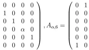
\[A _ {\alpha , 5} = \left( \begin{array}{c c c c c c} 0 & 1 & 0 & 0 & 0 & 0 \\0 & 0 & 1 & 0 & 0 & 0 \\0 & 0 & 0 & 1 & 0 & 0 \\0 & 0 & 0 & 0 & \alpha & 0 \\0 & 0 & 0 & 0 & 0 & 1 \\1 & 0 & 0 & 0 & 0 & 0 \end{array} \right), A _ {\alpha , 6} = \left( \begin{array}{c c c c c c} 0 & 1 & 0 & 0 & 0 & 0 \\0 & 0 & 1 & 0 & 0 & 0 \\0 & 0 & 0 & 1 & 0 & 0 \\0 & 0 & 0 & 0 & 1 & 0 \\0 & 0 & 0 & 0 & 0 & \alpha \\1 & 0 & 0 & 0 & 0 & 0 \end{array} \right).\]

The set is non-commutative. The set is another construction structures set of matrix solutions of the Diophantine equation associated to the matrix .

2.3 Construction Structures Set of Matrix Solutions of Diophantine Equations

Let be a positive integer. Assume that is a square matrix of order n and let introduce the associated construction structures set of matrix solutions. Let

\[A_{\alpha,1} = \left( \begin{array}{c c c c c c c c c} 0 & 1 & 0 & 0 & \dots & 0 & 0 & 0 & 0 \\0 & 0 & 1 & 0 & \dots & 0 & 0 & 0 & 0 \\0 & 0 & 0 & 1 & \dots & 0 & 0 & 0 & 0 \\0 & 0 & 0 & 0 & \dots & 0 & 0 & 0 & 0 \\\vdots & \vdots & \vdots & \vdots & \dots & \vdots & \vdots & \vdots & \vdots \\0 & 0 & 0 & 0 & \dots & 0 & 1 & 0 & 0 \\0 & 0 & 0 & 0 & \dots & 0 & 0 & 1 & 0 \\0 & 0 & 0 & 0 & \dots & 0 & 0 & 0 & 1 \\\alpha & 0 & 0 & 0 & \dots & 0 & 0 & 0 & 0 \end{array} \right)\]

be a Rare matrix of order and index 1. Denote by

\[A_{\alpha,2} = \left( \begin{array}{c c c c c c c c c} 0 & \alpha & 0 & 0 & \dots & 0 & 0 & 0 & 0 \\0 & 0 & 1 & 0 & \dots & 0 & 0 & 0 & 0 \\0 & 0 & 0 & 1 & \dots & 0 & 0 & 0 & 0 \\0 & 0 & 0 & 0 & \dots & 0 & 0 & 0 & 0 \\\vdots & \vdots & \vdots & \vdots & \dots & \vdots & \vdots & \vdots & \vdots \\0 & 0 & 0 & 0 & \dots & 0 & 1 & 0 & 0 \\0 & 0 & 0 & 0 & \dots & 0 & 0 & 1 & 0 \\0 & 0 & 0 & 0 & \dots & 0 & 0 & 0 & 1 \\1 & 0 & 0 & 0 & \dots & 0 & 0 & 0 & 0 \end{array} \right), A_{\alpha,3} = \left( \begin{array}{c c c c c c c c c} 0 & 1 & 0 & 0 & \dots & 0 & 0 & 0 & 0 \\0 & 0 & \alpha & 0 & \dots & 0 & 0 & 0 & 0 \\0 & 0 & 0 & 1 & \dots & 0 & 0 & 0 & 0 \\0 & 0 & 0 & 0 & \dots & 0 & 0 & 0 & 0 \\\vdots & \vdots & \vdots & \vdots & \dots & \vdots & \vdots & \vdots & \vdots \\0 & 0 & 0 & 0 & \dots & 0 & 1 & 0 & 0 \\0 & 0 & 0 & 0 & \dots & 0 & 0 & 1 & 0 \\0 & 0 & 0 & 0 & \dots & 0 & 0 & 0 & 1 \\1 & 0 & 0 & \dots & \dots & 0 & 0 & 0 & 0 \end{array} \right) ,\]
\[A _ {\alpha , 4} = \left( \begin{array}{c c c c c c c c c} 0 & 1 & 0 & 0 & \dots & 0 & 0 & 0 & 0 \\0 & 0 & 1 & 0 & \dots & 0 & 0 & 0 & 0 \\0 & 0 & 0 & \alpha & \dots & 0 & 0 & 0 & 0 \\0 & 0 & 0 & 0 & \dots & 0 & 0 & 0 & 0 \\\vdots & \vdots & \vdots & \vdots & \dots & \vdots & \vdots & \vdots & \vdots \\0 & 0 & 0 & 0 & \dots & 0 & 1 & 0 & 0 \\0 & 0 & 0 & 0 & \dots & 0 & 0 & 1 & 0 \\0 & 0 & 0 & 0 & \dots & 0 & 0 & 0 & 1 \\1 & 0 & 0 & 0 & \dots & 0 & 0 & 0 & 0 \end{array} \right),..., A _ {\alpha , n - 2} = \left( \begin{array}{c c c c c c c c c} 0 & 1 & 0 & 0 & \dots & 0 & 0 & 0 & 0 \\0 & 0 & 1 & 0 & \dots & 0 & 0 & 0 & 0 \\0 & 0 & 0 & 1 & \dots & 0 & 0 & 0 & 0 \\0 & 0 & 0 & 0 & \dots & 0 & 0 & 0 & 0 \\\vdots & \vdots & \vdots & \vdots & \dots & \vdots & \vdots & \vdots & \vdots \\0 & 0 & 0 & 0 & \dots & 0 & \alpha & 0 & 0 \\0 & 0 & 0 & 0 & \dots & 0 & 0 & 1 & 0 \\0 & 0 & 0 & 0 & \dots & 0 & 0 & 0 & 1 \\1 & 0 & 0 & 0 & \dots & 0 & 0 & 0 & 0 \end{array} \right),\]
\[A_{\alpha,n-1} = \left( \begin{array}{c c c c c c c c c} 0 & 1 & 0 & 0 & \dots & 0 & 0 & 0 & 0 \\0 & 0 & 1 & 0 & \dots & 0 & 0 & 0 & 0 \\0 & 0 & 0 & 1 & \dots & 0 & 0 & 0 & 0 \\0 & 0 & 0 & 0 & \dots & 0 & 0 & 0 & 0 \\\vdots & \vdots & \vdots & \vdots & \dots & \vdots & \vdots & \vdots & \vdots \\0 & 0 & 0 & 0 & \dots & 0 & 1 & 0 & 0 \\0 & 0 & 0 & 0 & \dots & 0 & 0 & \alpha & 0 \\0 & 0 & 0 & 0 & \dots & 0 & 0 & 0 & 1 \\1 & 0 & 0 & 0 & \dots & 0 & 0 & 0 & 0 \end{array} \right),\]

The set is called the construction structures set of matrix solutions of Diophantine equations. In this case, the set contains exactly 2n matrices.

2.4 Multiverses Associated to the Construction Structures Sets of Matrix Solutions of the Diophantine Equation

The Diophantine equation has an infinite number of construction structures sets of different sizes. In particular, matrices from the sets are matrix solutions of this Diophantine equation.

Definition 2.2. A multiverse (or parallel universes) is the collection of alternate universes that share a universal hierarchy.

Let be a construction structures set of matrix solution of the Diophantine equation . The set

\[\mathcal{M} = \{\mathcal{F}_{P_{\alpha}, Q_{\alpha}, H_{\alpha}}: P_{\alpha}, Q_{\alpha}, H_{\alpha} \in CS(A_{\alpha,1})\}\]

is called the multiverse of matrix triple solutions of the Diophantine equation . The set M is finite. We can now show that every multiverse of matrix triple solutions of the Diophantine equation is finite.

Proof of Theorem 1.1

We need to construct multiverses of matrix solutions elements of the set .

  • Assume that . In this case, the matrix solutions are elements of the set , we can consider the matrix
\[A_{\alpha ,1} = \left( \begin{array}{c c c c c c} 0 & 1 & 0 & 0 & 0 & 0 \\0 & 0 & 1 & 0 & 0 & 0 \\0 & 0 & 0 & 1 & 0 & 0 \\0 & 0 & 0 & 0 & 1 & 0 \\0 & 0 & 0 & 0 & 0 & 1 \\\alpha & 0 & 0 & 0 & 0 & 0 \end{array} \right)\]

and the construction structures set

\[C S _ {1} (A _ {\alpha , 1}) = \left\{A _ {\alpha , j}, A _ {\alpha , j} ^ {T}: j = 1, 2,..., 5, 6 \right\}\]

has 12 matrices. The universe

\[\mathcal{F}_{P_{\alpha},Q_{\alpha},H_{\alpha}} = \left\{\left(P_{\delta}^{2},Q_{\beta},H_{\delta+\beta}\right) : \delta,\beta\in\mathbb{N}\right\}, P_{\alpha},Q_{\alpha},H_{\alpha} \in CS_{1}(A_{\alpha,1})\]

is an infinite set. The set

\[\mathcal{M}_1 = \{\mathcal{F}_{P_{\alpha}, Q_{\alpha}, H_{\alpha}} : P_{\alpha}, Q_{\alpha}, H_{\alpha} \in CS_1(A_{\alpha, 1})\}\]

is called the first multiverse of matrix solutions of the equation

. This multiverse has exactly universes.

  • Assume that . Let
\[A_{\alpha , 1} = \left( \begin{array}{c c c c c c c c c c c c} 0 & 1 & 0 & 0 & 0 & 0 & 0 & 0 & 0 & 0 & 0 & 0 \\0 & 0 & 1 & 0 & 0 & 0 & 0 & 0 & 0 & 0 & 0 & 0 \\0 & 0 & 0 & 1 & 0 & 0 & 0 & 0 & 0 & 0 & 0 & 0 \\0 & 0 & 0 & 0 & 1 & 0 & 0 & 0 & 0 & 0 & 0 & 0 \\0 & 0 & 0 & 0 & 0 & 1 & 0 & 0 & 0 & 0 & 0 & 0 \\0 & 0 & 0 & 0 & 0 & 0 & 1 & 0 & 0 & 0 & 0 & 0 \\0 & 0 & 0 & 0 & 0 & 0 & 0 & 1 & 0 & 0 & 0 & 0 \\0 & 0 & 0 & 0 & 0 & 0 & 0 & 0 & 1 & 0 & 0 & 0 \\0 & 0 & 0 & 0 & 0 & 0 & 0 & 0 & 0 & 1 & 0 & 0 \\0 & 0 & 0 & 0 & 0 & 0 & 0 & 0 & 0 & 0 & 1 & 0 \\0 & 0 & 0 & 0 & 0 & 0 & 0 & 0 & 0 & 0 & 1 \end{array} \right)\]

be a Rare matrix of order 12 and index 1. The construction structures set

\[C S _ {2} (A _ {\alpha , 1}) = \left\{A _ {\alpha , j}, A _ {\alpha , j} ^ {T}: j = 1, 2,..., 1 1, 1 2 \right\}\]

has 24 matrices. The universe

\[\mathcal{F}_{P_{\alpha},Q_{\alpha},H_{\alpha}} = \left\{(P_{\delta}^{4},Q_{\beta}^{2},H_{\delta+\beta}^{2}): \delta,\beta \in \mathbb{N}\right\}, P_{\alpha},Q_{\alpha},H_{\alpha} \in CS_{2}(A_{\alpha,1})\]

is an infinite set. The set

\[\mathcal{M}_{2} = \{\mathcal{F}_{P_{\alpha}, Q_{\alpha}, H_{\alpha}} : P_{\alpha}, Q_{\alpha}, H_{\alpha} \in CS_{2}(A_{\alpha, 1})\}\]

is called the second multiverse of matrix solutions of the equation

. This multiverse has exactly universes.

  • Let be a positive integer and let
\[A_{\alpha,1} = \left( \begin{array}{c c c c c c c c c} 0 & 1 & 0 & 0 & \ldots & 0 & 0 & 0 & 0 \\0 & 0 & 1 & 0 & \ldots & 0 & 0 & 0 & 0 \\0 & 0 & 0 & 1 & \ldots & 0 & 0 & 0 & 0 \\0 & 0 & 0 & 0 & \ldots & 0 & 0 & 0 & 0 \\\vdots & \vdots & \vdots & \vdots & \ldots & \vdots & \vdots & \vdots & \vdots \\0 & 0 & 0 & 0 & \ldots & 0 & 1 & 0 & 0 \\0 & 0 & 0 & 0 & \ldots & 0 & 0 & 1 & 0 \\0 & 0 & 0 & 0 & \ldots & 0 & 0 & 0 & 1 \\\alpha & 0 & 0 & 0 & \ldots & 0 & 0 & 0 & 0 \end{array} \right) \in M_{6k}(\mathbb{N}), \alpha \neq 0,\]

be a Rare matrix of order 6k and index 1. Denote by

\[A _ {\alpha , 2} = \left( \begin{array}{c c c c c c c c c} 0 & \alpha & 0 & 0 & \dots & 0 & 0 & 0 & 0 \\0 & 0 & 1 & 0 & \dots & 0 & 0 & 0 & 0 \\0 & 0 & 0 & 1 & \dots & 0 & 0 & 0 & 0 \\0 & 0 & 0 & 0 & \dots & 0 & 0 & 0 & 0 \\\vdots & \vdots & \vdots & \vdots & \dots & \vdots & \vdots & \vdots & \vdots \\0 & 0 & 0 & 0 & \dots & 0 & 1 & 0 & 0 \\0 & 0 & 0 & 0 & \dots & 0 & 0 & 1 & 0 \\0 & 0 & 0 & 0 & \dots & 0 & 0 & 0 & 1 \\1 & 0 & 0 & 0 & \dots & 0 & 0 & 0 & 0 \end{array} \right), A _ {\alpha , 3} = \left( \begin{array}{c c c c c c c c c} 0 & 1 & 0 & 0 & \dots & 0 & 0 & 0 & 0 \\0 & 0 & \alpha & 0 & \dots & 0 & 0 & 0 & 0 \\0 & 0 & 0 & 1 & \dots & 0 & 0 & 0 & 0 \\0 & 0 & 0 & 0 & \dots & 0 & 0 & 0 & 0 \\\vdots & \vdots & \vdots & \vdots & \dots & \vdots & \vdots & \vdots & \vdots \\0 & 0 & 0 & 0 & \dots & 0 & 1 & 0 & 0 \\0 & 0 & 0 & 0 & \dots & 0 & 0 & 1 & 0 \\0 & 0 & 0 & 0 & \dots & 0 & 0 & 0 & 1 \\1 & 0 & 0 & \dots & \dots & 0 & 0 & 0 & 0 \end{array} \right)\]
\[A _ {\alpha , 4} = \left( \begin{array}{c c c c c c c c c} 0 & 1 & 0 & 0 & \ldots & 0 & 0 & 0 & 0 \\0 & 0 & 1 & 0 & \ldots & 0 & 0 & 0 & 0 \\0 & 0 & 0 & \alpha & \ldots & 0 & 0 & 0 & 0 \\0 & 0 & 0 & 0 & \ldots & 0 & 0 & 0 & 0 \\\vdots & \vdots & \vdots & \vdots & \ldots & \vdots & \vdots & \vdots & \vdots \\0 & 0 & 0 & 0 & \ldots & 0 & 1 & 0 & 0 \\0 & 0 & 0 & 0 & \ldots & 0 & 0 & 1 & 0 \\0 & 0 & 0 & 0 & \ldots & 0 & 0 & 0 & 1 \\1 & 0 & 0 & 0 & \ldots & 0 & 0 & 0 & 0 \end{array} \right), \ldots , A _ {\alpha , 6 k - 2} = \left( \begin{array}{c c c c c c c c c} 0 & 1 & 0 & 0 & \ldots & 0 & 0 & 0 & 0 \\0 & 0 & 1 & 0 & \ldots & 0 & 0 & 0 & 0 \\0 & 0 & 0 & 1 & \ldots & 0 & 0 & 0 & 0 \\0 & 0 & 0 & 0 & \ldots & 0 & 0 & 0 & 0 \\\vdots & \vdots & \vdots & \vdots & \ldots & \vdots & \vdots & \vdots & \vdots \\0 & 0 & 0 & 0 & \ldots & 0 ^ {\alpha} ^ {2} ^ {2} ^ {2} ^ {2} ^ {2} ^ {2} ^ {2} ^ {2} ^ {2} ^ {2} ^ {2} ^ {2} ^ {2} ^ {2} ^ {2} ^ {2} ^ {2} ^ {2} ^ {2} ^ {2} ^ {2} ^ {2} ^ {2} ^ {2} ^ {2} ^ {3} ^ {3} ^ {3} ^ {3} ^ {3} ^ {3} ^ {3} ^ {3} ^ {3} ^ {3} ^ {3} ^ {3} ^ {3} ^ {3} ^ {3} ^ {3} ^ {3} ^ {3} ^ {3} ^ {3} ^ {3} ^ {3} ^ {3} ^ {3} ^ {3} ^ {4} ^ {4} ^ {4} ^ {4} ^ {4} ^ {4} ^ {4} ^ {4} ^ {4} ^ {4} ^ {4} ^ {4} ^ {4} ^ {4} ^ {4} ^ {4} ^ {4} ^ {4} ^ {4} ^ {4} ^ {4} ^ {4} ^ {4} ^ {4} ^ {4} ^ {5} ^ {5} ^ {5} ^ {5} ^ {5} ^ {5} ^ {5} ^ {5} ^ {5} ^ {5} ^ {5} ^ {5} ^ {5} ^ {5} ^ {5} ^ {5} ^ {5} ^ {5} ^ {5} ^ {5} ^ {5} ^ {5} ^ {5} ^ {5} ^ {5} ^ {6} _ {\alpha^ {\prime}} A _ {\alpha , k - 2},\]
\[A_{\alpha,6k-1} = \left( \begin{array}{ccccccc} 0 & 1 & 0 & 0 & \dots & 0 & 0 \\0 & 0 & 1 & 0 & \dots & 0 & 0 \\0 & 0 & 0 & 1 & \dots & 0 & 0 \\0 & 0 & 0 & 0 & \dots & 0 & 0 \\\vdots & \vdots & \vdots & \vdots & \dots & \vdots & \vdots \\0 & 0 & 0 & 0 & \dots & 0 & 1 \\0 & 0 & 0 & 0 & \dots & 0 & 0 & \alpha & 0 \\0 & 0 & 0 & 0 & \dots & 0 & 0 & 0 & 1 \\1 & 0 & 0 & 0 & \dots & 0 & 0 & 0 & 0 \end{array} \right), A_{\alpha,6k} = \left( \begin{array}{ccccccc} 0 & 1 & 0 & 0 & \dots & 0 & 0 \\0 & 0 & 1 & 0 & \dots & 0 & 0 \\0 & 0 & 0 & 1 & \dots & 0 & 0 \\0 & 0 & 0 & 0 & \dots & 0 & 0 \\\vdots & \vdots & \vdots & \vdots & \dots & \vdots & \vdots \\0 & 0 & 0 & 0 & \dots & 0 & 1 \\0 & 0 & 0 & 0 & \dots & 0 & 0 & \alpha & 0 \\0 & 0 & 0 & 0 & \dots & 0 & 0 & 0 & 1 \\1 & 0 & 0 & 0 & \dots & 0 & 0 & 0 & 0 \end{array} \right)\]

It is well known that [5]. The set

\[CS_{k}(A_{\alpha,1}) = \{A_{\alpha,j}, A_{\alpha,j}^{T}: j = 1,2,...,6k\} \subset M_{6k}(\mathbb{N})\]

is the construction structures set of the matrix solutions of the Diophantine equation . The Diophantine equation

\[X^{6k} + Y^{6k} = Z^{6k},\]

allows us to deduce that

\[(X ^ {2 k}) ^ {3} + (Y ^ {k}) ^ {6} = (Z ^ {k}) ^ {6}.\]

Therefore,

\[(A _ {\alpha , j} ^ {2 k}) ^ {3} + (A _ {\beta , j} ^ {k}) ^ {6} = (A _ {\alpha + \beta , j} ^ {k}) ^ {6}, j = 1, 2,..., 6 k, \alpha , \beta \in \mathbb {N}.\]

The matrix triples , , satisfy the Diophantine equation . The universe

\[\mathcal{F}_{P_{\alpha}, Q_{\alpha}, H_{\alpha}} = \left\{\left(P_{\delta}^{2k}, Q_{\beta}^{k}, H_{\delta + \beta}^{k}\right) : \delta, \beta \in \mathbb{N}\right\}, P_{\alpha}, Q_{\alpha}, H_{\alpha} \in CS_{k}(A_{\alpha, 1}) \subset M_{6k}(\mathbb{N}),\]

is an infinite set. The set

\[\mathcal{M}_{k} = \{\mathcal{F}_{P_{\alpha}, Q_{\alpha}, H_{\alpha}}: P_{\alpha}, Q_{\alpha}, H_{\alpha} \in CS_{k}(A_{\alpha, 1})\}\]

is called the multiverse of matrix solutions of the Diophantine equation . The multiverse has

\[12k \times 12k \times 12k = 1728 \times k^{3}\]

universes of matrix solutions. This yields us the desired result.

Conflict of Interest

The authors declare no conflict of interest.

Ethical Approval

Not applicable

Data Availability

The datasets used in this study are openly available at [repository link] and the source code is available on GitHub at [GitHub link].

Funding

This work did not receive any external funding.

References

11 Cites in Article

Cite this article

Generating citation...

Related Research

  • MSC Code: 11D09, 15A03, 11C20
  • Version of record

    v1.0

  • Issue date

    15 July 2024

  • Language

    en

Article Placeholder
Open Access
Research Article
CC-BY-NC 4.0
Views 666
Downloads 26
Special Issue

Launch a focused special issue to highlight research, emerging trends, and expert insights in your academic field.

Support

