

IntelliPaper
Abstract
We developed a new theory of discriminant analysis (Theory1). Physicians can use it for practical medical diagnoses. Only Revised IP Optimal-LDF (RIP) obtains the minimum number of misclassification (MNM). RIP can discriminate linearly separable data (LSD) theoretically. It discriminated against 169 microarrays with two classes and found that 169 MNMs are zero and LSD. It can split high-dimensional arrays into many small LSD with less than n (patient’s number) genes that are the candidates of multivariate oncogenes. We completed a new theory of high-dimensional gene data analysis (Theory2). A 100-fold Cross-Validation (Method1) can rank all candidates for the importance of diagnosis. Thus, if physicians firstly use Theory2 as the screening method, they can start their medical studies with the correct small sizes of candidates. This paper analyzes four arrays in detail and proposes correctly choosing cancer and normal patients using four principles.
Explore Digital Article Text
I. INTRODUCTION
We completed a "New Discriminant Theory after R. A. Fisher (Theory1)" in 2015 [1-6]. After graduating from University, we worked at a private company and attended the project of the ECG diagnostic system at the Osaka Center for Cancer Cardiovascular Diseases (Center) and NEC. Dr. Nomura gave us ECG data over 1,000 patients having about 100 variables. These data (n÷1,000 * p÷100) consisted of one normal and over ten abnormal symptoms. He asked us to develop a diagnostic logic. From 1971 to 1974, we studied Fisher's linear discriminant function (LDF), quadratic discriminant function (QDF), and other statistical methods. We developed the diagnostic logic by LDF and QDF. Discriminant functions are weak for the discrimination of over three classes. We created several discriminant data with two classes, one normal symptom and one of the abnormal symptoms.
Our four-year study was inferior to Nomura's decision tree logic. This failure motivates us to develop the valuable discriminant theory for medical diagnosis. The number of misclassifications (NM) and error rate (ER) can evaluate discriminant results. However, those are unreliable because each discriminant functions have different NMs and ERs. Many defects of ER are the first problem of discriminant analysis (Problem1). We developed a Revised Optimal-LDF (RIP) that finds the minimum NM (MNM) that decreases monotonously . This fact is Fact2 of discriminant analysis. If MNM = 0, the data are linearly separable data (LSD). RIP by integer programming (IP) minimizes the NM and can find the MNM unique for the discriminant data. The first fact (Fact1) can explain the relation of LDF coefficients and NMs [1]. N linear equations made from n-cases divide the p-dimensional coefficients space into a finite convex polyhedron (CP). All interior points of each CP correspond infinite LDFs that have a unique NM = k and misclassify the same k-cases. There may be several optimal CPs (OCPs) having MNM. Only RIP can find one of the interior points of OCP theoretically. Therefore, RIP can quickly find 169 arrays are LSD. Because RIP can find the minimum ER, we need not compare many ERs of discriminant methods. Although many studies compare many ERs of classifiers, their efforts are useless.
RIP finds that Swiss banknote data consisting of 100 genuine and 100 counterfeit bills (200*6) [2, 6, 7] is LSD. A two variable model (x4, x6) is a minimum 2-dimensional LSD called a basic gene set (BGS) similar to Yamanaka's four genes. The 16 MNMs, including (x4, x6) among 63 models, are zero and LSD. The other 47 models are not LSD. We can explain this truth by Fact2. If is MNM having k-variables, several are the MNMs added one variable to the former k-variables. In the cancer gene data analysis (Theory2), Fact2 explains array has the Matryoshka data structure that includes small Matryoshkas in it up to BGS (Structure1). Thus, the array has huge multivariate oncogenes candidates. If physicians study the characteristic of BGS by oncogenes, we expect they can find the new meaning of multivariate oncogenes (Validation4).
All discriminant functions, except for RIP and hard margin SVM (H-SVM) [8], cannot correctly discriminate LSD theoretically. However, H-SVM cannot discriminate overlapping data by computational error. MNM=0 means the first statistic for LSD. We check all NMs of SMs and BGSs by eight discriminant functions. Because all NMs of logistic regression is zero, only logistic regression using the maximum-likelihood algorithm can discriminate LSD empirically. Except for three LDFs, other discriminant functions based on the variance-covariance matrices cannot discriminate LSD correctly. Because of no study of LSD discrimination (Problem2), most researchers do not know the exact meaning of LSD. Thus, all studies are wrong and useless for cancer gene diagnosis.
We realized all pass/fail determination of exams is naturally LSD [6]. However, some ERs of exams are over 30% by Fisher's LDF. QDF misclassifies all pass students into the failed class if all pass students correctly answer items. This truth is the defect of the generalized inverse matrix algorithm (Problem3). The discriminant theory is not inferential statistics (Problem4) because of no standard errors (SE) about discriminant coefficients and ER. We developed the 100-fold cross-validation (Method1) to estimate the experimental SE of both discriminant coefficients and ER. Many discriminant users validate their discriminant results by the leave-one-out method [9] or its extended k-fold CV. Both methods ignore the statistical principle of the relation of population and samples. Method1 is very easy and valuable. It copies the original data 100 times. That is the test sample and becomes the pseudo population. We add a random number to the test sample and sort it by the random values. We divide the sorted data into 100 training samples. Each training sample is a sample from the unique test sample. We call the averages of 100 ERs of training and test samples M1 and M2. M2=0 means that the original data and 100 test samples are LSD. We think SMs and BGSs with M2=0 are helpful for cancer diagnosis (Validation1).
After 1995, six medical projects studied the array profilings and released six first-generation arrays (old arrays) [10-15]. Many statisticians and engineers studied high-dimensional data analysis using these arrays. Because we completed Theory1 in 2015, we analyzed six old arrays downloaded from Higgins HP [16] as an applied problem of Theory1. RIP discriminated against six arrays and found those are LSD. Moreover, RIP could split six arrays into many Small Matryoshkas (SMs) within 54 days. Therefore, we completed the fundamental theory of gene data analysis (Theory2) until 2018 [17]. Until 2020, we confirmed six array results by 163 second-generation arrays (new arrays).
Because Theory1 and Theory2 are effortless and powerful, we expect medical specialists use those as a screening method at the entry point of medical diagnosis. Especially, SMs and BGSs with M2=0 become a beacon of medical research. This paper analyzes four arrays among 163 new arrays in detail and proposes the design principle of the array. Almost all analyses will finish in about one week.
II. MATERIAL AND METHOD
We explain materials and theories in three stages. Stages 1 introduces the summary of six old data, and Stages 2 introduces the summary of 73 arrays with two classes. Stages 3 introduces the new detailed analysis of four arrays among 73 arrays.
2.1 Six Old Arrays
Six medical projects have studied expression profiling of old arrays and published their papers. October 28 , 2015, we discriminated against Shipp data (77*7129) by RIP. RIP finds the MNM is zero, and Shipp array is LSD within one second.
Program1 is a program of the basic RIP coded by Mathematical Programming (MP) software named LINGO [18]. In [6], we explain RIP and Program1 in detail.
Moreover, we found that only 32 coefficients were not zero, and the other 7,097 coefficients were zero. We can naturally select 32 coefficients. Thus, other feature selection methods are useless. We can explain the reason for the surprising result by Fact1. Because Fact1 tells us the domain of RIP is less than n dimensions, RIP can find less than n=77 genes. We need to understand that the range of NM is [0, n] having integer values.
We call the 32 genes the first SM (SM1). In Theory2, we call LSD Matryoshka. We discriminated against 7,097 genes again and found the second SM2. We developed a Matryoshka feature selection method (Method2) and coded Program3 by LINGO explained in [17]. Program3 can split Shipp's array into 222 Type1 SMs (MNM=0) and one Type2 SM (MNM >= 1). Other studies find only one gene set, MNM of which is over 1. Those gene sets are not multivariate oncogenes
Table1 shows the summary of six arrays. The range of genes included in Type1 222 SMs is [18, 62]. MNM of Type2 SM is one and not LSD. JMP's logistic regression Degree of Freedoms (DF) range is [76, 80]. For the array , DF generally becomes almost the same patients' numbers instead of p. Thus, logistic regression can split the array into many DF gene sets with almost n genes (Structure4). All studies ignored this linear model principle restricted by the simultaneous solution condition. Only Golub arrays have SMs of 170 Type1 and 22 Type2. Type2's MNM range is [1, 24]. Most arrays have many Type1 SMs and one Type2 SM. No studies have found four data structures of LSD until now.
| n*p | Type1 | Genes | Range | Type2 (Genes) | MNM | DF | |
| Alon [10] | 62*2000 | 64 | 1,999 | [21, 42] | One SM with 1 gene | 25 | [61, 64] |
| Singh [14] | 102*12625 | 215 | 12,598 | [34, 85] | One SM with 27 genes | 25 | [85, 108] |
| Shipp [13] | 77*7129 | 222 | 7,085 | [18, 62] | One SM with 44 genes | 1 | [76, 80] |
| Tien [15] | 73*12625 | 101 | 12,566 | [100,139] | One SM with 59 genes | 4 | [172,180] |
| Chiaretti [11] | 128*12625 | 155 | 12,623 | [32, 122] | One SM with 2 genes | 47 | [99, 134] |
| Golub [12] | 72*7129 | 170 | 6,348 | [16, 56] | 22 SMs with 359 genes | [1,24] | [70, 75] |
Although many engineering researchers proposed feature selection methods (FSs), they found only one gene-set about 50 genes using one- or two-variables statistical methods. Their gene sets are not multivariate oncogenes and LSD. Furthermore, they ignored other genes as useless genes. Therefore, we concluded that all engineering studies have many mistakes and are useless for practical diagnosis [23]. Theory2 finds that array has four vital data structures:
Six arrays are LSD. Those have the Matryoshka data structure that includes much smaller LSD, up to BGS (Structure1).
We can split the array into many SMs (Structure2), BGSs (Structure3), and DF gene sets (Structure4).
Table 2 shows the validations of SMs by Method1. We summarize 170 SMs of Golub into five groups. MIN, MAX, and MEAN columns are the minimum, maximum, and average of 35 ERs of test samples. Because all NMs of training samples are zero, those are LSD. At first, we consider these results are promising. However, we find many test samples with M2=0 among SMs and BGSs of 163 new second-generation arrays registered on the GSE database after 2007. Thus, M2 can evaluate its important ranking of SMs and BGSs. Especially, SMs and BGSs with M2=0 are useful for diagnosis.
| MIN | MAX | MEAN (M2) | |
| SM1~SM35 | [0, 4.17] | [4.17, 18.1] | [0.42, 9.17] |
| SM36~SM70 | [0, 4.17] | [4.17,18.0] | [0.42, 9.17] |
| SM71~SM105 | [0, 9.72] | [8.33,23.6] | [5, 14.72] |
| SM106~SM140 | [1.39, 12.5] | [11.11, 25] | [7.08, 16.11] |
| SM141~SM170 | [0, 13.89] | [4.17,27.78] | [0.42, 18.89] |
Program4 split Alon's array into Type1 129 BGSs with 2,000 genes, and there are no Type2 BGSs. Table 3 shows the BGS3's results among 129 BGS by Method1. It consists of 22 normal subjects and 40 tumor patients. Although all 100 MNMs of training samples are zero, 100 test samples have three different results. NMs of the first samples are 4,000, which means that all cancers are misclassified into the normal. NMs of the 100th sample are 2,200, which means that all normal are misclassified into the tumors. Method1 is helpful in the multivariate candidate's evaluation, also. Because Alon selected 2,000 from 6,500 genes, we consider their FS to omit several essential genes.
| ...37 | ...100 | MIN | MAX | MEAN | ||
| Training Samples | 0 | 0 | 0 | 0 | 0 | 0 |
| Test Samples | 4000 | 900 | 2200 | 14.52 | 64.52 | 45.44 |
Program3 and 4 split Tien's array into 101 SMs and 561 BGSs, respectively. Physicians had found over 100 driver oncogenes and tumor suppressor genes. We count 100 oncogenes included in 101 SMs. One SM includes three oncogenes. Physicians can understand the meaning of this SM by three genes. Most SMs do not include oncogenesis. We propose this simple check as Validation4. Golub, Shipp, and Singh belonged at the same group of Harvard Institute. They used the weighted voting system for their original FS and selected about 50 genes included in the neighborhood of over k oncogenes. Although they consider the relation of their selected genes and the oncogenes, other researchers ignored these legacy oncogenes. We consider four validations of SMs and BGSs. Validation1 is M2 by Method1, and Validation2 is RatioSV. Validation3 is the check of Ward and PCA. Validation4 is the check of the legacy oncogenes included in BGSs. Validation5 uses the genome cohort.
We discriminated SMs and BGSs by eight LDFs and QDF. Those are six MP-based LDFs in addition to logistic regression and Fisher's LDF. SVM4 and SVM1 are the soft-margin SVM using the penalty c=10,000 and 1. Because the quadratic programming (QP) defines H-SVM, SVM4, and SVM1, non-zero coefficients are few. However, no studies have been conducted on why QP-LDFs are useless for FS. Table 4 shows the number of non-zero coefficients by six MP-based LDF.
In 2018, we completed the basic Theory2 by six old arrays. We developed Program3 and Program4, and RatioSV. Because RIP discriminant scores (RipDSs) show the malignancy indexes for diagnosis, we make a signal data having all RipDSs instead of genes. JMP [19], the statistical software, analyzes signal data instead of the high-dimensional array. We propose several medical research themes in [17].
| Alon(62*2,000) | Golub (72*7,129) | Shipp (77*7,129) | |
| RIP | 56 | 37 | 43 |
| IPLP | 34 | 19 | 31 |
| LP | 34 | 19 | 31 |
| H-SVM | 2000 | 6274 | 7124 |
| SVM4 | 2000 | 7129 | 7129 |
| SVM1 | 2000 | 6262 | 7123 |
2.2 The 73 additional arrays registered on CuMiDa Gene Database
Bruno et al. [20] developed a CuMiDa gene database that includes 78 arrays of 13 carcinomas registered on GSE gene DB after 2007. They selected these second-generation arrays after their quality check. It consists of five one-class arrays, 57 two-class arrays, and 16 with three to seven classes. We omit five one-class arrays from our analysis. We made 106 two-class arrays by two-class combinations from 16 data. Because we confirmed four data structures by 57 and 106 arrays, we completed Theory 2 [21-24] in 2022.
Table 5 shows the summary of 73 original arrays with over two classes. We show one or two arrays among 13 carcinomas. Type column shows the 13 carcinomas. GSE shows the GSE code. The n shows the number of cases. The case range is [12, 357] and 18 arrays have less than 30 cases. GENE shows Gene's number. Its range is [12621, 54676]. Because we wish to obtain the results quickly, we analyze 1,2621 genes, which are the maximum genes of six old arrays. R1 is the ratio of 1,2621 genes and all genes included in each array. Because Pancreatic and the sixth Brest6 contain 54,676 genes, two R1s are 0.23. Class means the 73 arrays' number of classes. We evaluated the first 10 SMs by Method1 (100-fold CV). MinM2 shows the minimum values of M2 of first 10 SMs. The range is [0, 12.24]. Because six old arrays have no SMs with M2=0, we consider the new arrays' quality of expression becomes better than old arrays. Otherwise, new arrays include more useful new genes for diagnosis. Nation shows the nation of the first author. LSD1 and LSD2 are the numbers of all SMs and BGSs with M2=0(10-fold CV). At first, we evaluate 10 SMs by 100-fold CV. Because the check of 100-fold CV is bothered, we evaluate all SMs and BGSs by the 10-fold CV. We use Table 5 for the becon of 169 arrays's analyses.
| ID | TYPE | GSE | n | GENE | R1 | CLASS | MinM2 | SVM | MLP | DT | NB | RF | Nation | LSD1 | LSD2 |
| Max | MAX | 357 | 54676 | 1 | 7 | 12.24 | 1 | 1 | 1 | 1 | 1 | 0 | 5 | 31 | |
| Min | MIN | 12 | 12621 | 0.231 | 2 | 0 | 0.26 | 0.29 | 0.25 | 0.34 | 0.34 | 0 | 0 | 0 | |
| Total | SUM | 5427 | 2867932 | 179 | 103.69 | 64.16 | 60.97 | 55.6 | 61.15 | 62.24 | 0 | 15 | 185 | ||
| 1 | Pancreatic | GSE16515 | 51 | 54676 | 0.23 | 2 | 0.45 | 0.86 | 0.78 | 0.78 | 0.84 | 0.82 | USA | 0 | 0 |
| 7 | Breast6 | GSE42568 | 116 | 54676 | 0.23 | 2 | 0 | 0.99 | 0.99 | 0.94 | 0.99 | 0.97 | Ireland | 0 | 2 |
| 17 | Liver3 | GSE14520 | 357 | 22278 | 0.57 | 2 | 0.11 | 0.97 | 0.8 | 0.92 | 0.96 | 0.96 | USA | 0 | 0 |
| 24 | Liver10 | GSE14520 | 41 | 22278 | 0.57 | 2 | 0 | 1 | 0.98 | 0.98 | 0.95 | 1 | USA | 0 | 7 |
| 25 | Throat1 | GSE42743 | 103 | 54676 | 0.23 | 2 | 0 | 0.87 | 0.83 | 0.85 | 0.86 | 0.87 | USA | 0 | 1 |
| 34 | Leuke mia6 | GSE28497 | 281 | 22284 | 0.57 | 7 | 0.88 | 0.72 | 0.73 | 0.78 | 0.79 | USA | |||
| 46 | Prostat e9 | GSE6919 | 124 | 12626 | 1.00 | 2 | 9.76 | 0.67 | 0.65 | 0.45 | 0.63 | 0.69 | USA | 0 | 0 |
| 51 | Ovary4 | GSE6008 | 98 | 22284 | 0.57 | 4 | 0.71 | 0.64 | 0.65 | 0.68 | 0.71 | USA | |||
| 52 | Brain1 | GSE50161 | 130 | 54676 | 0.23 | 5 | 0.02 | 0.95 | 0.82 | 0.85 | 0.85 | 0.91 | USA | 0 | 0 |
| 54 | Bladder1 | GSE31189 | 85 | 54676 | 0.23 | 2 | 12.24 | 0.64 | 0.58 | 0.54 | 0.46 | 0.55 | USA | 0 | 0 |
| 58 | Lung3 | GSE19804 | 114 | 54676 | 0.23 | 2 | 1.75 | 0.93 | 0.85 | 0.91 | 0.91 | 0.92 | Taiwan | 0 | 0 |
| 62 | Renal1 | GSE66270 | 28 | 54676 | 0.23 | 2 | 0 | 1 | 1 | 0.79 | 1 | 1 | Germany | 5 | 31 |
| 68 | Gastric3 | GSE19826 | 24 | 54676 | 0.23 | 2 | 0.04 | 0.67 | 0.67 | 0.67 | 0.71 | 0.67 | China | 0 | 0 |
| 74 | Colorectal6 | GSE8671 | 63 | 54676 | 0.23 | 2 | 0 | 1 | 1 | 0.94 | 1 | 1 | Swiss | 4 | 16 |
| 77 | Colorectal 9 | GSE21510 | 147 | 54676 | 0.23 | 3 | 0.99 | 1 | 0.9 | 0.97 | 0.94 | Japan |
Bruno et al. analyze original 78 arrays by the Weka program. They calculate eight classifiers' accuracy rates (1 - ERs) of all arrays. SVM, RF, Multilayer Perceptron, DT, Naïve Bayes are the supervised learning methods to analyze 73 supervised learning data. Because k-nearest neighbors, k-means, and Hierarchical Clustering are the unsupervised learning methods and are proper to analyze five one-class unsupervised learning data, we omit three ones from Table 5.
Because many engineering researchers use Weka, we can understand their results' overview by this table. Two (Mean ± SD) of SVM and RF are and . They recommend SVM and RF because both accuracy rates are better than others. Because the accuracy rates of Breast1 by SVM is 1, NM of SVM by three-fold CV is 0. If Weka's SVM is H-SVM, Breast1 is LSD. Because it is kernel-SVM, we cannot judge Breast1 is LSD or not. Thus, all classifiers cannot judge arrays are LSD or not because those discriminant hyperplanes are not linear. Only 16 arrays of 73 data can separate two-class by SVM. Because RIP finds all 163 arrays are LSD by 10-fold CV, we conclude that eight classifiers are useless for gene diagnosis.
Bruno's ER survey gives us a vital hint for the four categories of classifiers from the viewpoints of the reliability of ER or LSD discrimination.
First category: Only RIP, H-SVM, and logistic regression can correctly discriminate LSD.
Second category: NMs of statistical LDFs based on the variance-covariance matrices are unreliable, especially for LSD discrimination. Mostly, those are not zero. Six ERs of Chiaretti, Shipp, Alon, Singh, Golub, and Tien by Fisher's LDF using the singular value decomposition are 1%, 4%, 8%, 10%, 11%, and 17%, respectively.
Third category: QDF and kernel-SVM are non-linear discriminant functions. Even if NM is zero, it does not mean LSD. Fourth category: Because other classifiers such as the decision tree use the complex discriminant hyperplane, NM=0 does not mean LSD. We are afraid most researchers do not understand the correct definition of LSD. Although no researchers found LSD, we found many LSD. Those are Swiss banknote data, every exam data, Japanese 29 regular and 15 small cars, Fisher's Iris data [31], and 169 arrays.
Engineering researchers compare ERs of many classifiers and decide the best classifier for each data. Because RIP finds MNM and the minimum ER, we need not compare and select classifiers for LSD discrimination because RIP is the best theoretically [31]. If M2=0, it means that the original data, SMs and BGSs, training samples, and test samples are LSD. Now, MP-based LDFs, RIP and H-SVM, can discriminate LSD theoretically. JMP's logistic regression can discriminate LSD experimentally confirmed by over a thousand checks of SMs and BGSs.
Because we confirm four universal data structures by 169 arrays, we completed Theory2 in 2022.
2.3 Detail Study of Four Data
This paper analyzes four new arrays, Liver3 [26], Breast6 [27], Colorectal 6 [28], Renal 1 [29], precisely. We studied epidemiological data with Dr. Takaichirou Suzuki and others at the Center. We published many cancer diagnosis papers until 1983 [30]. Thus, we established three principles of patient design as follows:
Adequate sample size. Usually, statisticians think over 100 cases.
Equally sample sizes of both classes.
First analysis is to compare cancer with a control group. Physicians must analyze two different cancers after the first analysis. Although many arrays of 169 arrays ignore the above principles: 1) lack the normal class, 2) small sample size of fewer than 30 cases, 3) the unbalanced sample sizes.
These arrays do not obtain good data analysis results. We are suspicious that these projects do not expect vital gene data analysis results. However, we realize the fourth principle instead of the first principle by Liver3. Three projects, except for Colorectal6, have better modified their data by our advice and analyzed the modified array again. They will obtain many useful multivariate oncogenes within one week.
III. RESULT
3.1 Liver3
Liver3 consists of 181 HCC patients and 176 normal subjects. We expect a good result because it satisfies three principles: 1) Because the sample size is 357, it is enough data from a statistical viewpoint. Most statisticians expect over 100 cases. 2) The sizes of two-class are almost the same. 3) It has the normal control class. Moreover, it has the genome cohort for validation. However, we find the correct fourth principle only for gene expression. We consider Liver3 includes many specific patients interested in medical study. If physicians take those patients from the array and treat them as test samples, they can get better results by the medium sample. Or, they cangorize Liver 3 into several arrays.
Program3 split 12,671 genes into 89 SMs with 12,611 genes and SM90 with 60 genes (MNM=2) by 20 iterations of discrimination. CPU time is 2h13s. If Program3 discriminates twice, we obtain 40 SM with 12,615 by 8m22s. Because 40 SMs have many genes, we explain 89 SMs.
Table 6 shows 89 SMs' results by Method1. SM column shows the first 10 SMs. We omit other 79 results. Gene shows the gene's number of 10 SMs. The following three columns are the minimum, maximum, and average of 10 NMs for the test samples. The last three columns are the minimum, maximum, and averages of 10 ERs of test samples. However, last three rows are the summary of 89 SMs. M2 range is [0.18, 13.7] and the average is 5.1. There is no SMs with M2=0.
| SM | gene | min | max | mean | MIN | MAX | MEAN |
| 1 | 13 | 110 | 310 | 180 | 3.08 | 8.68 | 5.04 |
| 2 | 18 | 50 | 320 | 181 | 1.4 | 8.96 | 5.07 |
| 3 | 16 | 90 | 240 | 164 | 2.52 | 6.72 | 4.59 |
| 4 | 13 | 80 | 340 | 172 | 2.24 | 9.52 | 4.82 |
| 5 | 15 | 70 | 270 | 176 | 1.96 | 7.56 | 4.93 |
| 6 | 8 | 100 | 220 | 152 | 2.8 | 6.16 | 4.26 |
| 7 | 15 | 130 | 270 | 185 | 3.64 | 7.56 | 5.18 |
| 8 | 23 | 100 | 290 | 186 | 2.8 | 8.12 | 5.21 |
| 9 | 16 | 90 | 320 | 176 | 2.52 | 8.96 | 4.93 |
| 10 | 22 | 80 | 220 | 137 | 2.24 | 6.16 | 3.84 |
| MIN | 6 | 0 | 41 | 6.5 | 0 | 1.15 | 0.18 |
| MAX | 25 | 400 | 600 | 488 | 11.2 | 16.8 | 13.7 |
| Mean | 15 | 108 | 270.8 | 182.2 | 3.03 | 7.59 | 5.1 |
JMP uses two symbols and colors to identify cancer patients (×, Red) and normal subjects (○, Blue). Figure 1 shows Ward's two-way clustering (Left) and PCA (Right) of SM1. After the Ward analyzes SM1, PCA input the clustering color information. We strongly recommend these combinations analyses of both methods in Euclidean space. PCA has three plots. The middle scatter plot shows the most cancer patients on the first and fourth quadrants and the most normal subjects on the second and third quadrants. However, several cases overlap with another class. The cumulative contribution ratio of the first and second components is 23.73 (=16.5+7.23)%. It explains about 24% variation out of 357 cases variation. The left plot shows the eigenvalues, and the right plot shows the factor loading plot. Ward has three parts. The left part shows the 357 cases. The middle part is the two-way clustering. The right part is the case dendrogram. The bottom dendrogram shows the variable dendrogram. Although the upper red part corresponds to cancer patients and the lower blue part corresponds to the normal subjects, several cases are misclassified to another class like PCA's scatter plot. We strongly recommend taking off misclassified cases that may be specific cases from the analysis and treating those cases as test samples.
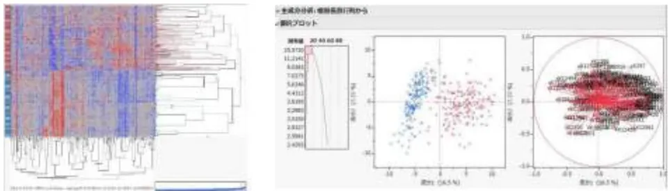
Figure 2 shows SM89's 357 cases located in 138-dimensional gene space. The scatter plot shows that both cases overlap near the origin. Two classes locate on four quadrants, and the cumulative contribution ratio is . Because all SMs are LSD, we know two classes are separable in the other 136-dimensional subspace. However, we consider that physicians do not use SM89 for diagnosis by Validation3 judgement.
We strongly recommend taking off these misclassified cases found in Figure 1. The omitted cases are helpful for the validation of Theory2's result as same as the gene cohort. If researchers analyze the modified arrays, they can obtain more precise results from SM1.
{"image_source":{"path":"images/bcd029f8ac9d17de8bdfb8adb0c3ef76976722b1926752b768c7ec76c62a6c22.jpg"},"content":"","chart_caption":[{"type":"text","content":"Figure 2: Ward cluster (Left figure) and PCA (Right figure) of SM89 of Liver (GSE14568)"}],"chart_footnote":[]}
We split 12,561 genes included in 89 SMs into BGSs by Program4. However, we stopped this work. We must calculate each BGS one by one, and it needs about two days. Because SM1's results are wrong, BGS brings no merit for diagnosis. If we confirm the excellent results of Method1 after Ward and PCA (Validation3), we had better obtain the BGS.
3.2 Breast6
Breast6 consists of 101 cancer patients and 15 normal subjects. Although the total case number is 116, we can forecast the bad results because the normal cases are few. If this project collects more than 35 normal subjects and selects 50 typical cancer patients, they can get marvelous results by 100 cases.
Program3 split 12,671 genes into 113 SMs with 12,618 genes and SM114 with 53 genes (MNM=1) by twice discrimination. CPU time is 6m29s. If Program3 discriminates 20 times, CPU time is 3h42m 16s. We obtain 359 SMs with 12,646 genes. Table 7 shows the results of 114 SMs by Method1. SM column shows only 13 SMs and SM114. The min, max, mean show three values of MNM of ten test samples. MIN, MAX, and MEAN are three values of ERs of ten test samples. There is no SMs with M2=0. The last three rows show the summary of 114 SMs. The range of 114 minimum, maximum and average values are [0, 7.8], [7.8, 21.55], and [4, 15], respectively. Results are bad because of the unbalanced data.
| SM | min | max | mean | MIN | MAX | MEAN |
| 1 | 30 | 230 | 93 | 2.688 | 20.61 | 8.333 |
| 2 | 10 | 210 | 89 | 0.896 | 18.82 | 7.975 |
| 3 | 20 | 90 | 48 | 1.792 | 8.065 | 4.301 |
| 4 | 10 | 100 | 45 | 0.896 | 8.961 | 4.032 |
| 5 | 40 | 180 | 99 | 3.584 | 16.13 | 8.871 |
| 6 | 30 | 220 | 114 | 2.688 | 19.71 | 10.22 |
| 7 | 30 | 170 | 102 | 2.688 | 15.23 | 9.14 |
| 8 | 30 | 190 | 82 | 2.688 | 17.03 | 7.348 |
| 9 | 40 | 160 | 94 | 3.584 | 14.34 | 8.423 |
| 10 | 30 | 130 | 85 | 2.688 | 11.65 | 7.616 |
| 111 | 90 | 250 | 174 | 7.759 | 21.55 | 15 |
| 112 | 30 | 140 | 79 | 2.586 | 12.07 | 6.81 |
| 113 | 30 | 140 | 82 | 2.586 | 12.07 | 7.069 |
| 114 | 10 | 140 | 60 | 0.862 | 12.07 | 5.172 |
| MIN | 0 | 90 | 45 | 0 | 7.759 | 4.032 |
| MAX | 90 | 250 | 174 | 7.759 | 21.55 | 15 |
| Mean | 20.53 | 143.8 | 73.74 | 1.778 | 12.44 | 6.382 |
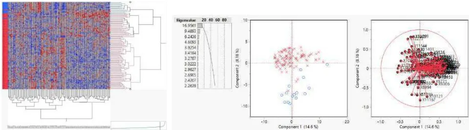
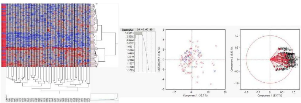
Figures 3 and 4 show both figures of SM1 and SM113. Figure 4 shows 101 cancer patients gathered around the origin. If we do not know the two classes' labels, we consider 15 normal subjects to be outliers of 101 patients. Normal subjects become the subset of cancer because of the small sample size. If the normal sample size is almost the same, we consider both classes more separable (Validation3). However, because these are our hypotheses, we must need further study.
Most researchers misunderstand the class information. Only discriminant functions can analyze the class information. Other statistical methods can analyze only the measured variables, not classified information, and those use the class information as a label.
Figures 3 and 4 show three clustering pairs and fourteen clustering pairs. According to clustering results, two classes of the scatter plot are almost overlapping.
We consider the unbalanced sizes to cause this problem.
{"image_source":{"path":"images/054966c51fbbfe3b155124a4ab2fb887ecf3f6636ea4cbe58b9ca8f97f160908.jpg"},"content":"","chart_caption":[],"chart_footnote":[]} {"image_source":{"path":"images/37ddcdbe5c48339705805fc14474f3c1d860d36d8a793e103fd9d3bbf3d6aefe.jpg"},"content":"","chart_caption":[],"chart_footnote":[]}
{"image_source":{"path":"images/5b789501913052fecb21afa0c795e72e4c9e6e5c870df5cfe1e9a978620de975.jpg"},"content":"","chart_caption":[],"chart_footnote":[]} {"image_source":{"path":"images/4fbab23338c7537cf91f2050095f75035f85861d2838348a3cc7cc586033ff9d.jpg"},"content":"","chart_caption":[{"type":"text","content":"Figure 4: The two-way clustering and PCA of SM113 of Breast (GSE42568)"},{"type":"text","content":"3.3 Colorectal6"}],"chart_footnote":[]}
Colorectal6 consists of 31 adenoma patients and 32 normal subjects. We doubt a good result because of less than 100 cases. Program3 split the array into 543 SMs with 12,609 genes and SM544 with 12 genes (MNM=3). Although Method1 evaluates 544 SMs, Table 8 shows 14 SMs with M2=0 and the other five SMs. The last column is RatioSV (Validation2). Because the result is better than Liver3 and Breast6, we consider the medium sample size is better than over 100 cases.
| SM | gene | min | max | mean | MIN | MAX | MEAN | min | max | mean | MIN | MAX | MEAN | RatioSV |
| 1 | 13 | 0 | 0 | 0 | 0 | 0 | 0 | 0 | 0 | 0 | 0 | 0 | 0 | 37.368 |
| 2 | 18 | 0 | 0 | 0 | 0 | 0 | 0 | 0 | 30 | 10 | 0 | 4.7619 | 1.5873 | 44.147 |
| 3 | 16 | 0 | 0 | 0 | 0 | 0 | 0 | 0 | 0 | 0 | 0 | 0 | 0 | 52.927 |
| 17 | 13 | 0 | 0 | 0 | 0 | 0 | 0 | 0 | 0 | 0 | 0 | 0 | 0 | 41.707 |
| 20 | 11 | 0 | 0 | 0 | 0 | 0 | 0 | 0 | 0 | 0 | 0 | 0 | 0 | 39.023 |
| 23 | 6 | 0 | 0 | 0 | 0 | 0 | 0 | 0 | 0 | 0 | 0 | 0 | 0 | 23.022 |
| 24 | 15 | 0 | 0 | 0 | 0 | 0 | 0 | 0 | 0 | 0 | 0 | 0 | 0 | 39.078 |
| 40 | 9 | 0 | 0 | 0 | 0 | 0 | 0 | 0 | 0 | 0 | 0 | 0 | 0 | 32.497 |
| 45 | 11 | 0 | 0 | 0 | 0 | 0 | 0 | 0 | 0 | 0 | 0 | 0 | 0 | 26.214 |
| 50 | 11 | 0 | 0 | 0 | 0 | 0 | 0 | 0 | 0 | 0 | 0 | 0 | 0 | 16.627 |
| 53 | 12 | 0 | 0 | 0 | 0 | 0 | 0 | 0 | 0 | 0 | 0 | 0 | 0 | 20.968 |
| 54 | 17 | 0 | 0 | 0 | 0 | 0 | 0 | 0 | 0 | 0 | 0 | 0 | 0 | 39.879 |
| 106 | 18 | 0 | 0 | 0 | 0 | 0 | 0 | 0 | 0 | 0 | 0 | 0 | 0 | 32.224 |
| 141 | 11 | 0 | 0 | 0 | 0 | 0 | 0 | 0 | 0 | 0 | 0 | 0 | 0 | 24.246 |
| 165 | 14 | 0 | 0 | 0 | 0 | 0 | 0 | 0 | 0 | 0 | 0 | 0 | 0 | 28.344 |
| 541 | 45 | 0 | 0 | 0 | 0 | 0 | 0 | 110 | 160 | 134 | 17.46 | 25.397 | 21.27 | - |
| 542 | 38 | 0 | 0 | 0 | 0 | 0 | 0 | 80 | 170 | 131 | 12.698 | 26.984 | 20.794 | - |
| 543 | 41 | 0 | 0 | 0 | 0 | 0 | 0 | 100 | 140 | 121 | 15.873 | 22.222 | 19.206 | - |
| 544 | 12 | 0 | 2 | 0.7 | 0 | 3.17 | 1.11 | 3 | 150 | 77 | 4.7619 | 23.81 | 12.222 | - |
| MIN | 6 | 0 | 0 | 0 | 0 | 0 | 0 | 0 | 0 | 0 | 0 | 0 | 0 | - |
| MAX | 48 | 0 | 2 | 1.3 | 0 | 3.17 | 2.06 | 110 | 200 | 134 | 17.46 | 31.746 | 21.27 | - |
| Mean | 23.2 | 0 | 0.05 | 0.02 | 0 | 0.03 | 0.01 | 15.8 | 65.3 | 36.7 | 2.5152 | 10.361 | 5.8252 | - |
{"image_source":{"path":"images/a5c42f539be0bfa01fa3449082e1d776599c939e0708672509f0cf4923698539.jpg"},"content":"","chart_caption":[{"type":"text","content":"Figure 5: Ward cluster (Left figure) and PCA of SM1 of Colorectal (GSE8671)"}],"chart_footnote":[]}
Figure 6 shows SM543's figures. Ward cluster shows two classes become 18 small clusters. The scatter plot shows two classes overlap. Although the cumulative contribution ratio is the scatter plot cannot show LSD. Although two classes become LSD on other 10-dimensional space, it is useless for diagnosis. Validation3 is useful for selecting vital multivariate oncogenes.
{"image_source":{"path":"images/f6a36888fe24ad746b1451c0b7fbe1359c6c07bacc1c77418257967aec314da1.jpg"},"content":"","chart_caption":[{"type":"text","content":"Figure 6: Ward cluster (Left figure) and PCA of SM89 of Colorectal (GSE8671)"}],"chart_footnote":[]}
3.4 Renal1
We never recommend the following analysis for arrays having less than 30 cases. If researchers agree with our claim, they collect about an additional 30 patients and analyze the same with Colorectal6. Renal1 consists of 14 normal subjects and 14 cancer patients. Although Renal1 does not satisfy Principle1, we misunderstood that the analysis of Renal1 is easy because of the small sample at first. Thus, we analyzed it step by step by Theory2 in detail. However, we spent two weeks and got awful results.
Program3 quickly splits the first 12,621 genes into 1,066 SMs (MNM=0) and the last SM1067 with one gene (MNM=14). Here, we had better stop the analysis and estimate the final SMs as follows. Because the average of genes included in 1066 SMs is 11.83 and Renal1 has 54,676 genes, it may consist of about 4,618 SMs. We had better estimate the number of SMs.
However, we skipped the above estimate. Next, Program4 split the genes included in 1,066 SMs into BGSs. After obtaining both results, we evaluated both SMs and BGSs by Method1. Physicians never follow this procedure, especially for a small sample. Physicians analyze case-by-case. For small samples, we recommend the following steps. SM decomposition is easy. Next, Program4 split the genes contained in SM1 into BGS, as shown in Table 9. Then, Method1 evaluates SM1 and 8 BGSs. We consider other small samples' results may be wrong as same as the table. This analysis' results show two critical facts. The numbers of genes of 6 BGSs are one, and the other two BGSs are 3. This result means that six single-genes can easily discriminate 28 patients into six LSDs.
| RIP | Gene | min | max | mean | MIN | MAX | MEAN |
| SM1 | 12 | 1400 | 1400 | 1400 | 50 | 50 | 50 |
| BGS11 | 1 | 1400 | 1400 | 1400 | 50 | 50 | 50 |
| BGS12 | 1 | 1400 | 1400 | 1400 | 50 | 50 | 50 |
| BGS13 | 1 | 1400 | 1400 | 1400 | 50 | 50 | 50 |
| BGS14 | 1 | 1400 | 1400 | 1400 | 50 | 50 | 50 |
| BGS15 | 1 | 1400 | 1400 | 1400 | 50 | 50 | 50 |
| BGS16 | 3 | 1400 | 1400 | 1400 | 50 | 50 | 50 |
| BGS17 | 1 | 1400 | 1400 | 1400 | 50 | 50 | 50 |
| BGS18 | 3 | 1400 | 1400 | 1400 | 50 | 50 | 50 |
However, Method1 tells us that NMs and ERs of 100 test samples are very bad. As shown by the minimum, maximum, and average values, 1400 cases, which is half of the 2,800 cases, are misclassified, and all Minimum, Maximum, and Average ERs are 50%. M2=50 becomes the stopping rule of M2 for small data. Although most researchers use a k-fold CV, they cannot obtain the same severe result as Method1. Fig. 7 shows two figures by Ward and PCA of SM1. Because the results are so good, this project have better added cancer and normal patients by the same criteria. If the results are wrong, they must change the patient selection criterion.
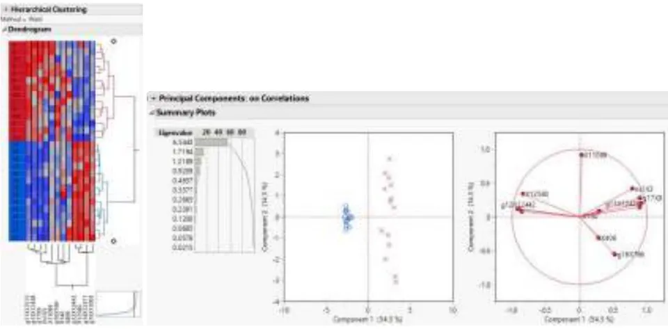
It is important that only Colorectal6 has good results in Validation1 and Validation3. Now, we cannot decide the proper threshold of RatioSV (Validation2).
IV. DISCUSSION
Theory1 solved four discriminant problems by RIP and Method1. NM and ER evaluate discriminant results. Thus, we developed RIP that finds MNM. Because discriminant analysis is not inferential statistics and ER is the most vital statistics defined by class information, we found two vital facts of discriminant analysis. Fact1 tells us the relation of LDF coefficients and NM. Only RIP finds MNM that decreases monotonously (Fact2). Therefore, RIP can easily find LSD and confirms that 169 arrays are LSD. RIP can split the array into many SMs and BGSs. At last, we find Fact3 that 169 arrays have four universal data structures similar to many Matryoshka nested dolls [31].
This paper analyzes four arrays, such as Liver3, Breast6, Colorectal6, and Renal1. We consider Liver3 includes several specific patients important from the medical study. In general, we expect the best results of Liver3 that satisfy three design principles of cancer and normal subjects. However, Validation1 (Method1) and two figures (Validation3) tell us the problems.
Program3 and 4 find many SMs and BGSs candidates of multivariate oncogenes. Method1 (Validation1) gives us the vital ranks of diagnosis, especially M2=0. Because our screening methods by Theory1 and Theory2 almost finish within one week, every physician analyzes their DNA and RNA gene data as the screening methods at the first study before medical research. They can save much research time and obtain many correct multivariate oncogenes LSD. We completed the discriminant theory of LSD useful for all discriminant data [31] in 2023.
We sincerely hope physicians will achieve to overcome cancer by our methods.
ACKNOWLEDGMENT
Our research depends on the powerful LINGO solver supported by L. Schrage, K. Cunningham, and H. Ichikawa (LINDO Japan). We could establish Theory2 by IP solver and statistical software using suitable arrays. J. Sall developed JMP, a powerful statistical package. Bruno et al. developed CuMiDa. Jeffery et al. uploaded six old data. Thanks also for the suppliers of 73 medical studies. The late father's legacy, Otojirou, was helpful in these studies.
Conflict of Interest
The authors declare no conflict of interest.
Ethical Approval
Not applicable
Data Availability
The datasets used in this study are openly available at [repository link] and the source code is available on GitHub at [GitHub link].
Funding
This work did not receive any external funding.
References
Cite this article
Related Research

Special Issue
Launch a focused special issue to highlight research, emerging trends, and expert insights in your academic field.