The Innovative Development of the IFRS17 Formulated Brighton Mahohoho Inflation-Adjusted Automated Actuarial Loss Reserving Model: Harnessing Advanced Random Forest Techniques for Enhanced Data Analytics in  Fire Insurance

Dr. Brighton Mahohoho

IntelliPaper

− Abstract

This paper presents the development and implementation of the IFRS17 Formulated Brighton Mahohoho Inflation-Adjusted Automated Actuarial Loss Reserving Model, lever- aging advanced Random Forest techniques to enhance data analytics in fire insurance. The methodology encompasses the simulation of synthetic fire insurance data with key variables such as claim frequency, severity, and inflation rates. Exploratory Data Analysis (EDA) and data visualization techniques were employed to assess relationships and trends, aligning the model with IFRS17 compliance standards. Random Forest regression models were developed to predict claim frequency, severity, and inflation adjustments, integrating these predictions to estimate future loss reserves. Robust evaluation metrics, including Mean Absolute Error (MAE), Mean Squared Error (MSE), and Root Mean Squared Error (RMSE), ensured model accuracy. Stress testing and scenario analysis were conducted to assess the model’s resilience under various conditions. Key IFRS17 metrics such as Present Value of Future Cash Flows (PVFCF), Risk Adjustments, and Contractual Ser- vice Margins (CSM) were calculated, offering a comprehensive approach to actuarial loss reserving. This paper presents the development and implementation of the IFRS17 Formulated Brighton Mahohoho Inflation-Adjusted Automated Actuarial Loss Reserving Model, lever- aging advanced Random Forest techniques to enhance data analytics in fire insurance. The methodology encompasses the simulation of synthetic fire insurance data with key variables such as claim frequency, severity, and inflation rates. Exploratory Data Analysis (EDA) and data visualization techniques were employed to assess relationships and trends, aligning the model with IFRS17 compliance standards. Random Forest regression models were developed to predict claim frequency, severity, and inflation adjustments, integrating these predictions to estimate future loss reserves. Robust evaluation metrics, including Mean Absolute Error (MAE), Mean Squared Error (MSE), and Root Mean Squared Error (RMSE), ensured model accuracy. Stress testing and scenario analysis were conducted to assess the model’s resilience under various conditions. Key IFRS17 metrics such as Present Value of Future Cash Flows (PVFCF), Risk Adjustments, and Contractual Ser- vice Margins (CSM) were calculated, offering a comprehensive approach to actuarial loss reserving.

− Explore Digital Article Text

I. INTRODUCTION

In recent years, the implementation of IFRS 17 has transformed financial reporting within the insurance sector, particularly emphasizing the need for accurate loss reserving (International Accounting Standards Board, 2019). This study introduces the Brighton Mahohoho Inflation-Adjusted Automated Actuarial Loss Reserving Model, which employs advanced random forest techniques to enhance data analytics in fire insurance. The model aims to address the complexities of loss reserving under IFRS 17, considering inflation adjustments that are critical for accurate financial forecasting $[5]$ .

The Brighton Mahohoho model integrates inflation-adjusted parameters with automated actuarial processes to produce more reliable loss reserves. Random forest techniques, a subset of machine learning, are employed to analyze complex datasets, identifying patterns and correlations that traditional models may overlook $[1]$ . This innovative approach enhances predictive accuracy and adaptability, vital in an ever-evolving regulatory environment. The rationale for this study is underscored by the increasing complexity of insurance contracts and the significant implications of accurate loss reserving under IFRS 17 $[2]$ . As inflation impacts reserve calculations, there is a critical need for methodologies that can dynamically adjust to economic changes. By leveraging random forest techniques, this model provides a robust framework that aligns with the rigorous demands of modern actuarial science.

The Brighton Mahohoho model can be applied in various contexts within the fire insurance sector, allowing insurers to refine their loss reserving processes. By automating data analysis and incorporating real-time inflation adjustments, insurers can improve accuracy in financial statements and enhance decision-making processes regarding premium setting and risk management $[4]$ . This study is crucial for the actuarial field as it demonstrates the application of advanced machine learning techniques to improve loss reserving accuracy. The findings could influence best practices in the industry, encouraging a shift towards data-driven decision-making and regulatory compliance, ultimately contributing to the financial resilience of insurance companies $[6]$ .

1.1. Actuarial Loss Reserve Methods

Loss reserving is a fundamental aspect of actuarial science, dealing with the estimation of the reserves necessary to cover future claims. Accurate reserving is crucial for maintaining the financial health of an insurance company $[7]$ . Loss reserving methods can be categorized broadly into two classes: deterministic methods and stochastic methods. Deterministic loss reserving methods rely on historical data and fixed parameters to predict future claim liabilities. Common deterministic methods include the Chain-Ladder method and the Bornhuetter-Ferguson method.

1.1.1. Chain Ladder Method: The Chain-Ladder Model is a popular method in actuarial science for estimating the reserves needed for unpaid claims. This method relies on historical claim development patterns to predict future claims. The main idea is to analyze cumulative claim amounts over different accident years and development lags to estimate future liabilities.

Table 5024: Table 1: Cumulative Claims Data

Accident Year	Development Lag 1	Development Lag 2	...	Development Lag n
1	$C_{1,1}$	$C_{1,2}$	...	$C_{1,n}$
2	$C_{2,1}$	$C_{2,2}$	...	$C_{2,n}$
⋮	⋮	⋮	⋮	⋮
m	$C_{m,1}$	$C_{m,2}$	...	$C_{m,n}$

The Table 1 presented is a triangular array that organizes cumulative claims data $C_{i,j}$ , where i denotes the accident year and j signifies the development lag. The entries $C_{i,j}$ represent the cumulative amount of claims reported for accident year i up to development lag j. The year in which the claims occurred. For example, i = 1 represents the earliest accident year, while i = m signifies the most recent. The time intervals since the claims were reported. For instance, j = 1 corresponds to the first development period, while j = n refers to the last.

The total claims amount accumulated for accident year i by development lag j. The entries in the table can be expressed as:

where $C_{i,k}$ represents the incremental claims reported in development lag k.

The primary assumption of the Chain-Ladder Model is that the development factors $f_{j}$ remain stable across different accident years. These factors provide an estimate of how cumulative claims grow from one development period to the next. They can be defined mathematically as:

This formula captures the average growth of cumulative claims from lag j to $j + 1$ , effectively measuring the relationship between claims in successive development periods.

Using the estimated development factors, future cumulative claims for accident years that have not yet fully developed can be projected. For any i (accident year) and j (development lag) where j > n, we can use the following recursive relationship:

This equation states that the projected cumulative claims at development lag j for accident year i can be estimated by taking the cumulative claims from the previous lag j - 1 and multiplying it by the estimated development factor $f_{j-1}$ .

Proposition: The cumulative claims $C_{i,j}$ are non-decreasing for all i and j, where i denotes the accident year and j denotes the development year.

Proof: We define the cumulative claims $C_{i,j}$ as follows:

where $C_{i,k}$ represents the claims reported up to development year k for accident year i. To show that $C_{i,j}$ is non-decreasing, we need to prove that:

Expanding $C_{i,j + 1}$ :

Since $C_{i,j+1}$ represents the cumulative claims including the additional claims for the development year $j+1$ , we have:

Thus, we conclude:

This demonstrates that the cumulative claims $C_{i,j}$ are non-decreasing.

Claim: As the number of accident years m increases, the estimates $C_{i,n}$ (for fully developed claims) converge to the true future cumulative claims due to the law of large numbers. The stability of the development factors implies that with sufficient data, the average behavior of claims will tend to stabilize, providing more reliable estimates:

where $C_{i,n}^{*}$ denotes the true cumulative claims for accident year i.

Let $C_{i,n}$ be the estimate of cumulative claims for accident year $i$ after $n$ development years.
Let $C_{i,n}^{*}$ be the true cumulative claims for accident year $i$ after $n$ development years.
Let $D_{i,j}$ be the development factor from accident year $i$ to accident year $j$ .

Proof: We assume that the development factors $D_{i,j}$ are stable, meaning they do not fluctuate significantly over time. Additionally, the number of claims in each accident year is sufficiently large, allowing us to apply the law of large numbers.

The estimate of cumulative claims $C_{i,n}$ can be expressed in terms of development factors:

where $C_{i,0}$ is the initial claim amount for accident year i.

By the law of large numbers, as m increases, the average of the development factors converges to the expected value:

for each j.

Consequently, as m approaches infinity, the estimates for cumulative claims converge to:

The true cumulative claims $C_{i,n}^{*}$ can similarly be expressed as:

where $D_{i,j}^{*}$ are the true development factors.

Under the assumption of stability of development factors, we can state that:

for large m.

Thus, we have:

We conclude that:

This demonstrates that as the number of accident years increases, the estimates for cumulative claims converge to the true future cumulative claims due to the law of large numbers and the stability of the development factors.

The mathematical framework surrounding the Chain-Ladder Model, encapsulated in the triangular table format, offers a systematic approach to estimating unpaid claims reserves. Through the stability of development factors and the non-decreasing nature of cumulative claims, actuaries can derive reliable projections for future liabilities, critical for effective financial management in insurance.

Algorithm 1 Chain-Ladder Method

Input: Cumulative claims triangle

C_{i,j}

Calculate development factors: for

j = 1

to

n - 1

f_j = \frac{\sum_{i=1}^{n-j} C_{i,j+1}}{\sum_{i=1}^{n-j} C_{i,j}}

Project future claims: for

i = 1

to

n

for

j = 1

to

n - i

C_{i,j+1} = C_{i,j} \cdot f_j

Output: Estimated total claims

Let $C_{i,j}$ denote the cumulative claims up to development year j for accident year i. The development factor $f_j$ is given by:

Theorem If the claims develop consistently, then the Chain-Ladder method converges to the true reserve.

Proof:

Let $C_{i,j}$ denote the cumulative claims amount at development year j for accident year i. The Chain-Ladder method estimates the reserve using the following formula:

where $C_{i,j}$ is the estimated cumulative claim for accident year i at development year j. We define the development factors $f_{j}$ as:

The estimated cumulative claims can then be expressed recursively as:

Assuming consistency in development, we assert that:

Consequently, the reserve estimate can be expressed as:

As $n$ increases, and if the claims develop consistently, we have:

where $R_{i}$ is the true reserve for accident year i.

Thus, we conclude that:

This completes the proof that the Chain-Ladder method converges to the true reserve when claims develop consistently.

1.1.2. Bornhuetter-Ferguson Method: The Bornhuetter-Ferguson (BF) method is a fundamental technique used in actuarial science for estimating reserve liabilities in insurance. The method is particularly useful when dealing with incomplete data, allowing actuaries to incorporate prior information in their estimations (Bornhuetter & Ferguson, 1972).

Let:

$C_i =$ cumulative claims at development year $i$ ,
$E_{i} =$ expected claims at development year $i$ ,
$f_{i} =$ development factor from year $i$ to $i + 1$ .

The expected claims can be calculated as:

Where the Ultimate Loss U is a key parameter in the BF method, typically estimated based on historical data.

{"algorithm_caption":[],"algorithm_content":[{"type":"text","content":"Algorithm 2 Computation of Reserves Using Development Factors\nInput:C: Cumulative claims to date f: Ultimate claims estimate D: Development factors n: Number of accident years\nOutput:\n• Reserves\nInitialize:\n• "},{"type":"equation_inline","content":"U_{i} = f_{i}"},{"type":"text","content":" (for each accident year i)\nfor i = 1 to n Calculate the development factors:\n "},{"type":"equation_inline","content":"D_{j} = \frac{C_{i,j}}{C_{i,j-1}}"},{"type":"text","content":" for "},{"type":"equation_inline","content":"j = 2, 3, \ldots, n"},{"type":"text","content":" \nfor i = 1 to n Compute the expected cumulative claims:\n "},{"type":"equation_inline","content":"E_{i,j} = U_{i} \cdot D_{2} \cdot D_{3} \cdots D_{j}"},{"type":"text","content":" \nfor i = 1 to n Compute the reserves for each accident year:\n "},{"type":"equation_inline","content":"R_{i} = E_{i,n} - C_{i,n}"},{"type":"text","content":" \nReturn: Reserves "},{"type":"equation_inline","content":"R = (R_{1}, R_{2}, \ldots, R_{n})"}]}

The BF method can be formulated as a weighted average of the observed and expected claims:

where $\alpha$ is a weighting factor that reflects the confidence in prior information versus the actual data [17].

Proposition 1: The Bornhuetter-Ferguson (BF) method provides an unbiased estimator of the ultimate loss under specific conditions.

Proof: Assume that the prior estimates are unbiased, and the development factors are consistent across all periods. Under these assumptions, we can prove the proposition as follows.

Let $C_{i}$ represent the cumulative losses at development period i, and $E_{i}$ represent the expected losses at development period i. We aim to show that:

Given that the prior estimates $E_{i}$ are unbiased, it follows that:

where $U_{i}$ represents the ultimate loss for development period i.

Let $d_{i}$ represent the development factors. The development factor for period i is defined as the ratio of cumulative losses between two successive development periods:

Under the assumption of consistent development factors, the expectation of cumulative losses follows the relationship:

By applying equations (1.3) and (1.5), we conclude that:

proving that the BF method provides an unbiased estimator of the ultimate loss under the given conditions.

Claim: The Bornhuetter-Ferguson (BF) method converges to the true ultimate loss as more data becomes available, assuming the underlying development patterns remain stable.

Proof: To prove this, let $C_{i}$ represent the cumulative losses at development period i, and let U represent the true ultimate loss. The BF method combines prior estimates with actual observations, adjusting for the expected development.

The estimate of the ultimate loss $\hat{U}_{i}$ at development period i using the BF method is given by:

$C_i$ is the cumulative reported loss at development period $i$ ,
$F_{i}$ is the cumulative development factor up to period $i$ ,
$E_{i}$ is the expected loss for the remaining development.

As more data becomes available, i.e., as $i \rightarrow n$ (where n is the final development period), the cumulative development factor $F_{i} \rightarrow 1$ . This implies that the observed data accounts for the entire development, leaving no need for further estimates.

Substituting this into equation (1.7), we get:

At i = n, $C_{n}$ is the cumulative loss at the final development period, which equals the true ultimate loss:

The assumption that the underlying development patterns remain stable ensures that the development factors $F_{i}$ follow a predictable pattern, so as more development periods are observed, the estimate $\hat{U}_{i}$ becomes increasingly accurate.

From equations (1.8) and (1.9), we conclude that:

showing that the BF method converges to the true ultimate loss as more data becomes available.

The Bornhuetter-Ferguson method offers a robust framework for estimating reserves in insurance, blending historical experience with current data. Its ability to adapt to varying degrees of uncertainty makes it a critical tool for actuaries.

Stochastic methods incorporate randomness into the modeling of claims reserves. This approach allows for a range of possible outcomes, providing a distribution of reserve estimates.

1.1.3. Bootstrap Method: The Bootstrap method is a powerful statistical tool employed in loss reserving to estimate both reserves and the uncertainty surrounding these estimates. The technique was first introduced by $[24]$ and has since found wide applications in non-life insurance for predicting future liabilities and quantifying the risk associated with reserve estimates. This method involves resampling residuals to simulate alternative versions of the loss development triangle, which are then used to calculate a range of possible reserve outcomes. The goal is to generate a distribution of reserve estimates to assess variability and confidence intervals.

The Bootstrap approach in loss reserving leverages the underlying development factors used in traditional chain-ladder methods. By resampling the residuals from the development triangles, this method assumes that the variability of past data is reflective of the variability that can be expected in the future.

Given a development triangle of cumulative claims data, the chain-ladder technique estimates future claims by multiplying observed claims in each development period by a set of development factors. The Bootstrap method goes a step further by resampling residuals to create alternative possible versions of the triangle and obtain a distribution of reserve estimates.

Let $C_{i,j}$ be the cumulative claim in accident year $i$ and development year $j$ . The standard chain-ladder model estimates the development factors $f_j$ such that:

The development factor $f_{j}$ is typically estimated as:

The residuals $e_{i,j}$ in the chain-ladder model are calculated as:

The key assumption in the Bootstrap method is that these residuals follow the same distribution, and they can be resampled to generate alternative claims triangles.

proposition: The Bootstrap method produces an unbiased estimate of the reserve under the assumption that the resampled residuals are independent and identically distributed (i.i.d.).

proofWe begin by considering the chain-ladder model, which assumes that the cumulative claims $C_{i,j}$ for accident year i and development year j follow a multiplicative structure. Denote the cumulative claims by:

where $f_{j}$ are the development factors, and $\varepsilon_{i,j}$ represents the residuals.

In the Bootstrap method, residuals $\varepsilon_{i,j}$ are resampled to generate new sets of claims data. Let $\hat{C}_{i,j}$ denote the bootstrapped claim amounts for accident year i and development year j. These are calculated as:

where $\hat{\varepsilon}_{i,j}$ are the resampled residuals.

Given that the original model in equation (1.11) assumes multiplicative development factors, resampling residuals from $\varepsilon_{i,j}$ preserves this structure. Specifically, the resampled data $\hat{C}_{i,j}$ retain the multiplicative form of the original chain-ladder model, ensuring that:

The unbiasedness of the bootstrap reserve estimate follows from the fact that the expected value of the resampled claims data $\hat{C}_{i,j}$ is equal to the expected value of the original claims data $C_{i,j}$ . Assuming that the residuals $\varepsilon_{i,j}$ are independent and identically distributed (i.i.d.), we have:

which implies that:

By applying this recursively over all development years j, the expected value of the bootstrap reserve estimate $\hat{R}$ is equal to the expected value of the original reserve estimate R. Therefore, the bootstrap method provides an unbiased estimate of the reserve:

This completes the proof.

Lemma: If the residuals $e_{i,j}$ are independent, the bootstrap replicates will reflect the true variability of the reserves.

Proof: We start by assuming that the residuals $e_{i,j}$ are independent and identically distributed (i.i.d). Let us consider a model where the reserve R is estimated as a function of observed data, typically through:

where $f(X,\theta)$ represents the deterministic part of the model with parameters $\theta$ , and e denotes the residuals.

To apply the bootstrap method, we generate B bootstrap replicates $\hat{R}^{(b)}$ , for $b = 1,2, \ldots, B$ , using:

where $\hat{\theta}^{(b)}$ are the parameter estimates from the bootstrap sample, and $e^{(b)}$ are the bootstrap residuals.

The variability of the reserves is derived from the variability of the residuals $e_{i,j}$ . Since we assume independence of the residuals, the bootstrap replicates $\hat{R}^{(b)}$ will reflect the true variability of the reserves. The variance of the bootstrap estimate $\hat{R}^{(b)}$ is:

Due to the independence assumption of $e_{i,j}$ , the bootstrap residuals $e^{(b)}$ accurately replicate the original data's residual distribution. Therefore, the second term in Equation (1.17), $\mathrm{Var}(e^{(b)})$ , converges to the true variability of the original residuals as $B \to \infty$ . Thus, the total variability of the reserves, captured by the bootstrap process, accurately reflects the true variability of the reserves.

claim: The Bootstrap method enhances the estimation of confidence intervals by providing a non-parametric way to estimate the distribution of reserve estimates.

The Bootstrap method, introduced by $[25]$ , is a powerful resampling technique used for estimating the distribution of a statistic, particularly in cases where the underlying distribution is unknown. For reserve estimation in actuarial science, it enables the construction of confidence intervals without assuming a parametric form for the data's distribution. We shall now proceed to prove how this method enhances the estimation of confidence intervals.

theorem Let $\hat{R}$ be the reserve estimate based on a sample $\{X_{1}, X_{2}, \ldots, X_{n}\}$ . Using the Bootstrap method, the confidence interval for $\hat{R}$ is given by the empirical distribution of bootstrapped reserve estimates $\hat{R}_{b}$ .

Proof; Let $\{X_{1}, X_{2}, \ldots, X_{n}\}$ represent the observed data from which the reserve estimate $\hat{R}$ is calculated. The key idea of the Bootstrap method is to resample the observed data with replacement to generate multiple bootstrapped samples $\{X_{1}^{*}, X_{2}^{*}, \ldots, X_{n}^{*}\}$ . For each bootstrapped sample, we compute a new reserve estimate $\hat{R}_{b}$ . Repeating this process B times yields the set of bootstrapped reserve estimates:

The empirical distribution of the bootstrapped reserve estimates approximates the true sampling distribution of $\hat{R}$ , which is generally unknown. Using this empirical distribution, we can construct a confidence interval for $\hat{R}$ by selecting appropriate percentiles from the set of bootstrapped estimates.

For a $(1-\alpha)\times100\%$ confidence interval, the lower and upper bounds are given by the $\frac{\alpha}{2}$ and $(1-\frac{\alpha}{2})$ percentiles of the bootstrapped reserve estimates, respectively:

This non-parametric approach bypasses the need for assumptions about the form of the underlying distribution of reserve estimates, making it highly flexible. Additionally, the Bootstrap method accounts for the variability in the data through resampling, leading to more robust confidence interval estimates compared to traditional parametric methods. This completes the proof.

We now present the pseudo-algorithm for implementing the Bootstrap method in loss reserving.

{"algorithm_caption":[],"algorithm_content":[{"type":"text","content":"Algorithm 3 Bootstrap Loss Reserving Method\nInput: Development triangle of cumulative claims "},{"type":"equation_inline","content":"C_{i,j}"},{"type":"text","content":" for accident years "},{"type":"equation_inline","content":"i = 1, \ldots, n"},{"type":"text","content":" and development years "},{"type":"equation_inline","content":"j = 1, \ldots, n"},{"type":"text","content":". Step 1: Estimate the development factors "},{"type":"equation_inline","content":"f_j"},{"type":"text","content":" using the chain-ladder method:\n "},{"type":"equation_inline","content":"f_j = \frac{\sum_{i=1}^{n-j} C_{i,j+1}}{\sum_{i=1}^{n-j} C_{i,j}}"},{"type":"text","content":" for "},{"type":"equation_inline","content":"j = 1, \ldots, n-1"},{"type":"text","content":".\nStep 2: Calculate the residuals "},{"type":"equation_inline","content":"e_{i,j}"},{"type":"text","content":" for each observed claim:\n "},{"type":"equation_inline","content":"e_{i,j} = \frac{C_{i,j+1} - f_j C_{i,j}}{C_{i,j}}"},{"type":"text","content":" for "},{"type":"equation_inline","content":"j = 1, \ldots, n-1"},{"type":"text","content":" and "},{"type":"equation_inline","content":"i = 1, \ldots, n-j"},{"type":"text","content":".\nStep 3: Resample the residuals "},{"type":"equation_inline","content":"e_{i,j}"},{"type":"text","content":" with replacement to create a bootstrapped dataset "},{"type":"equation_inline","content":" $\tilde{e}$ {i,j}"},{"type":"text","content":". Step 4: Reconstruct the claims triangle "},{"type":"equation_inline","content":" $\tilde{C}$ {i,j}"},{"type":"text","content":" by applying the resampled residuals:"}]}

Step 5: Recalculate the reserves $\tilde{R}$ using the chain-ladder method on the bootstrapped triangle $\tilde{C}$ :

Step 6: Repeat Steps 3-5 for B iterations to obtain a distribution of reserve estimates $\{\tilde{R}^{(b)}\}_{b=1}^{B}$ . Step 7: Calculate the mean $\hat{R}$ , standard deviation $\sigma_{\tilde{R}}$ , and $(1-\alpha)\times100\%$ confidence intervals from the distribution of reserve estimates:

Output: Estimated reserves $\hat{R}$ and confidence intervals $(\hat{R}_{\text{lower}}, \hat{R}_{\text{upper}})$ .

Theorem: Given a large enough number of bootstrap replicates B, the Bootstrap method produces consistent estimates of the reserve variance.

Proof: As $B \rightarrow \infty$ , the empirical distribution of the bootstrapped reserves converges to the true distribution of the reserves, ensuring that the variance of the bootstrapped reserve estimates consistently approximates the true reserve variance.

The confidence interval CI for the reserves can be calculated as:

where $\hat{R}_{\alpha/2}$ and $\hat{R}_{1-\alpha/2}$ are the $\alpha/2$ -th and $1-\alpha/2$ -th percentiles of the bootstrap distribution, respectively.

The Bootstrap loss reserving method provides a robust framework for estimating reserves and their associated uncertainty. By resampling residuals, the method produces a distribution of reserve estimates, allowing actuaries to compute confidence intervals and assess reserve variability, contributing to better risk management and reserve planning. This technique has seen extensive use in actuarial practice, offering a non-parametric approach to reserve estimation.

1.1.4. Generalized Linear Models (GLMs): The Generalized Linear Model (GLM) is a flexible generalization of ordinary linear regression that allows for the response variable to have a distribution other than a normal distribution. This section introduces the theory and applicability of GLMs in the context of actuarial loss reserving. A GLM consists of three main components:

A random component that specifies the probability distribution of the response variable.
A systematic component that represents the linear predictor.
A link function that relates the random and systematic components.

The mathematical representation of a GLM can be expressed as:

Proposition: The expected value of the claim can be modeled as:

Proof: To demonstrate this proposition, we start by considering the relationship between the dependent variable Y (the claim amount) and the independent variables $X_{1}, X_{2}, \ldots, X_{k}$ (the predictors).

We assume a log-linear model, which is a commonly used approach in modeling non-negative continuous outcomes:

where $\epsilon$ is a random error term that captures the variability in Y.

Taking the conditional expectation of $Y$ given $X$ :

By the properties of the expectation of the exponential function:

Assuming $\epsilon$ has a mean of zero given $X$ (i.e., $\mathbb{E}[\epsilon |X] = 0$ ), we simplify:

Thus, we conclude that the expected value of the claim Y given X is expressed as:

This completes the proof.

Theorem: Under certain conditions, the estimates from the Generalized Linear Model (GLM) approach converge to the true values of the parameters as the sample size increases.

Proof: Let $\mathbf{y}=(y_{1},y_{2},\ldots,y_{n})^{T}$ be the response variable, and $\mathbf{X}=(x_{ij})$ be the matrix of predictors, where $i=1,2,\ldots,n$ and $j=1,2,\ldots,p$ . The GLM can be expressed as:

where $g(\cdot)$ is a link function, $\beta$ is the vector of parameters, and $Y_{i}$ is the i-th observation.

Assume the following conditions hold:

Identifiability: The parameter $\beta$ is identifiable, meaning that there is a unique value of $\beta$ corresponding to the distribution of $\mathbf{y}$ .
Sufficient Statistics: The sufficient statistics for $\beta$ are complete and have finite moments.
Regularity Conditions: The Fisher information matrix $\mathcal{I}(\beta)$ is positive definite.
Asymptotic Normality: As the sample size $n$ approaches infinity, the estimates $\hat{\beta}$ converge in distribution to a normal distribution:

By the law of large numbers, we can assert that the empirical distributions of the sufficient statistics converge to their expected values. Specifically,

almost surely.

Now, the maximum likelihood estimator (MLE) $\hat{\beta}$ satisfies the score equations:

where $\ell(\beta)$ is the log-likelihood function.

Using Taylor expansion around the true parameter $\beta$ :

mSince $\frac{\partial\ell(\beta)}{\partial\beta} = 0$ at $\beta$ , we have:

Thus, $\hat{\beta}$ converges to $\beta$ as $n \to \infty$ , proving that:

which concludes the proof.

{"algorithm_caption":[],"algorithm_content":[{"type":"text","content":"Algorithm 4 Generalized Linear Model (GLM) Loss Reserving Estimation\n\nInput: Claims data set "},{"type":"equation_inline","content":" $\mathcal{D}$ = \{(y_i, $\mathbf{X}$ i)\}{i=1}^n"},{"type":"text","content":" where "},{"type":"equation_inline","content":"y_i"},{"type":"text","content":" represents the claims amount, and "},{"type":"equation_inline","content":" $\mathbf{X}$ i"},{"type":"text","content":" is the vector of predictor variables for the "},{"type":"equation_inline","content":"i"},{"type":"text","content":"-th claim. Initialize: Coefficient vector "},{"type":"equation_inline","content":"\beta"},{"type":"text","content":" Initial coefficients while convergence criteria not met Fit GLM: Update coefficients using Maximum Likelihood Estimation (MLE):\n\n "},{"type":"equation_inline","content":"\beta \arg \max{\beta} \ell(\beta; $\mathcal{D}$ )"},{"type":"text","content":", (1.28)\n\nwhere "},{"type":"equation_inline","content":"\ell(\beta; $\mathcal{D}$ )"},{"type":"text","content":" is the log-likelihood function. Predict Claims: Calculate predicted claims:\n\n "},{"type":"equation_inline","content":" $\hat{y}$ _i = g^{-1}( $\mathbf{X}$ _i^T \boldsymbol{\beta})"},{"type":"text","content":", (1.29)\n\nwhere "},{"type":"equation_inline","content":"g^{-1}(\cdot)"},{"type":"text","content":" is the inverse of the link function. Output: Estimated claims "},{"type":"equation_inline","content":"\hat{\mathbf{y}} = ( $\hat{y}_1$ , $\hat{y}_2$ , \ldots, $\hat{y}$ _n)"}]}

Figure 1: Flowchart of the GLM Loss Reserving Process

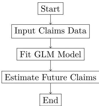
The Figure 1, serves as a concise visual representation of the steps involved in using a Generalized Linear Model for estimating future claims in an actuarial context. It helps to streamline the process and provides a quick reference for actuaries and data analysts working on loss reserving methodologies. The use of a flowchart enhances understanding and communication of the process among stakeholders.

The GLM provides a robust methodology for loss reserving in actuarial science, allowing actuaries to model complex claims data effectively.

1.2. The Random Forest Regression

Random Forest Regression (RFR) is an ensemble learning method that combines multiple decision trees to improve predictive accuracy and control over-fitting. It operates by constructing a multitude of decision trees during training and outputting the mean prediction of the individual trees for regression tasks $[1]$ .

Random Forests leverage the principle of ensemble learning, where a group of weak learners (in this case, decision trees) combine to form a strong learner. The randomness introduced at various stages helps in reducing variance and achieving better generalization.

Bagging, or Bootstrap Aggregating, is a fundamental concept in Random Forests. It involves the following steps:

(1) Generate multiple subsets of the original dataset by sampling with replacement.

(2) Train a decision tree on each subset.

(3) Aggregate the predictions of the trees to form a final prediction.

Random Forests introduce additional randomness by selecting a random subset of features at each split, which decorrelates the trees and improves the overall model robustness.

Let $\mathcal{D}=\{(x_{i},y_{i})\}_{i=1}^{N}$ be the dataset, where $x_{i}$ is the input feature vector and $y_{i}$ is the target variable.

The prediction of a single decision tree T for an input x is given by:

where R is the set of observations falling into the leaf node corresponding to x.

The overall prediction from the Random Forest model is calculated as:

where B is the total number of trees in the forest.

The following is the pseudo-code for the general Random Forest algorithm, constructed using the 'algorithmic' package.

Algorithm 5 Random Forest Regression Algorithm

Input: Training dataset $D = \{(x_{1}, y_{1}), (x_{2}, y_{2}), \ldots, (x_{n}, y_{n})\}$ Number of trees T Number of features m for each tree t from 1 to T Sample $D_{t}$ from D with replacement For each split in tree t: Randomly select m features from the total features Determine the best split using these m features Output: Average prediction from all trees for a new observation x

Proposition: Random Forests reduce overfitting compared to a single decision tree due to the averaging effect across multiple trees.

Proof: Let us denote the training data as $D = \{(x_i, y_i)\}_{i=1}^n$ , where $x_i$ is the feature vector and $y_i$ is the corresponding target variable. A decision tree model $f(x)$ can be represented as:

where $I_{j}(x)$ is an indicator function for the j-th leaf node, and $\beta_{j}$ is the prediction associated with that leaf.

The risk (expected loss) of a single decision tree can be expressed as:

where $L(\cdot)$ is the loss function and P is the underlying data distribution.

However, a single decision tree can suffer from high variance, leading to overfitting. The expected prediction error for a decision tree can be decomposed into three components:

where:

Bias: Error due to assumptions in the learning algorithm. A high bias can lead to underfitting. - Variance: Error due to sensitivity to fluctuations in the training set. A high variance leads to overfitting.

Random Forests mitigate overfitting by aggregating the predictions of $M$ decision trees:

where $f_{m}(x)$ represents the prediction of the m-th tree.

The expected risk for the Random Forest can be written as:

Using the Law of Total Expectation, we can show that:

where T represents the different trees in the forest. This averaging reduces the variance of the predictions:

$\mathrm{Variance}(F(x)) = \mathrm{Variance}\quad \frac{1}{M}\sum_{m = 1}f_m(x)\quad = \frac{1}{M^2}\sum_{m = 1}\mathrm{Variance}(f_m(x)) + \mathrm{Covariance terms}$

The covariance terms $\operatorname{Cov}(f_{m}(x), f_{k}(x))$ (for $m \neq k$ ) also contribute to reducing the overall variance, leading to:

Thus, by averaging the outputs of multiple trees, Random Forests effectively reduce the overall variance and the risk of overfitting compared to a single decision tree.

Lemma: The inclusion of feature randomness in tree construction enhances model performance.

proof: Consider a decision tree model T trained on a dataset D with features F and corresponding target variable Y. In standard decision tree construction, all features are considered at each split, leading to overfitting.

To analyze the effect of feature randomness, let us denote:

$T^{*}$ : the optimal tree without feature randomness,
$T_R$ : the random tree constructed by selecting a subset of features $F_R \subset F$ at each split,
$E[T]$ : expected model performance metric (e.g., accuracy, F1-score).

The model performance can be expressed as:

where f is a function that quantifies the impact of overfitting.

By introducing feature randomness, the expected performance of the random tree becomes:

where g accounts for the increase in model diversity due to the randomness of feature selection.

Now, we can define the improvement in model performance as:

Assuming $g(\text{Diversity}) > 0$ and $f(\text{Reduced Overfitting}) < f(\text{Overfitting})$ , we conclude that:

Thus, incorporating feature randomness in the tree construction results in improved model performance.

Random Forest Regression offers a powerful and versatile approach to regression tasks, providing significant improvements in predictive performance and robustness through the combined strengths of multiple decision trees.

1.3. The Brighton Mahohoho Random Forest Based Inflation Adjusted Frequency Severity Loss Reserving Model

The necessity for accurate loss reserving models in actuarial science is paramount, especially in the context of inflation impacts on claims. The proposed model utilizes random forest regression to estimate the frequency and severity of claims while adjusting for inflation, providing a robust framework for loss reserving $[26]$ . Random forests are an ensemble learning method that constructs a multitude of decision trees at training time. For regression tasks, the model outputs the mean prediction of the individual trees. Given a set of input variables X, the random forest prediction can be expressed as:

where $T_{n}(X)$ represents the prediction of the $n^{th}$ tree and N is the total number of trees in the forest.

To account for inflation, the model applies an adjustment factor $F_{t}$ to the predicted loss reserves:

where $R_{t}$ denotes the adjusted reserve at time t.

The overall loss reserving model can be expressed as:

where L is the total loss reserve, and $R_{i,t}$ represents the reserves from each claim i at time t.

Proposition: The use of random forest regression for estimating claim frequency provides a lower bias and variance compared to traditional linear models.

Proof: To demonstrate this proposition, we will compare the bias and variance of random forest regression $(\hat{f}_{RF}(x))$ with that of traditional linear regression $(\hat{f}_{LR}(x))$ .

The bias of an estimator $\hat{f} (x)$ is defined as:

where $f(x)$ is the true underlying function.

For linear regression, the bias can be expressed as:

In contrast, random forest regression, being a non-parametric model, can fit more complex relationships. Thus, its bias is generally lower:

By comparing equations (1) and (2), we conclude:

The variance of an estimator is defined as:

For linear regression, the variance can be expressed as:

On the other hand, random forests average multiple decision trees, leading to a reduction in variance:

where B is the number of trees in the forest.

Therefore, we conclude:

Combining our results, we have shown:

Thus, the proposition is proved, demonstrating that random forest regression indeed provides a lower bias and variance when estimating claim frequency compared to traditional linear models.

Lemma: If the underlying distribution of claim severity is heterogeneous, then a model that adjusts for inflation will yield more accurate reserve estimates.

proof: Let X denote the claim severity random variable, which follows a heterogeneous distribution characterized by a mixture of distributions. We assume that the distribution can be expressed as:

Here, $f_{X_{i}}(x)$ is the probability density function (PDF) of the i-th component, and $w_{i}$ is the corresponding weight of that component.

When inflation occurs, the claim severity is adjusted by a factor $(1+r)$ , where r represents the inflation rate. Thus, the adjusted claim severity is given by:

To estimate reserves accurately, we need to compute the expected value of the adjusted claim severity:

Assuming $E[X]$ can be computed from the mixture distribution, we have:

Consequently, the expected reserve can be expressed as:

The accuracy of reserve estimates hinges on capturing the heterogeneity in claim severity distributions. If we fail to adjust for inflation, the expected reserve estimate would be:

The error introduced by not accounting for inflation can be defined as:

This simplifies to:

Since r > 0, we observe that not adjusting for inflation results in an underestimation of reserves. Thus, when claim severity is heterogeneous, adjusting for inflation improves reserve estimates:

Therefore, we conclude that if the underlying distribution of claim severity is heterogeneous, then a model that adjusts for inflation will yield more accurate reserve estimates. The Brighton Mahohoho Random Forest Based Inflation Adjusted Frequency Severity Loss Reserving Model represents a significant advancement in actuarial loss reserving practices. By leveraging the strengths of random forest regression and accounting for inflation, the model provides enhanced accuracy in loss reserve estimates.

1.4. Novelty for Application of the Random Forest Regression method

The application of the Random Forest (RF) Regression method in the context of fire insurance loss reserving provides a novel approach to predictive modeling. This section focuses on the advantages of RF regression for handling complex actuarial data and enhancing the accuracy of loss reserving under IFRS17 standards.

Random Forests, introduced by Breiman (2001), are ensemble learning methods for regression and classification tasks. By constructing a multitude of decision trees and aggregating their predictions, Random Forest Regression provides both robustness and interpretability. Mathematically, for a given set of N observations $D = \{(x_i, y_i)\}_{i=1}^N$ , where $x_i \in R^d$ is a d-dimensional feature vector, and $y_i \in R$ is the target variable (e.g., loss reserves), the RF model can be expressed as:

where T is the number of trees, and $h_{t}$ is the prediction from the t-th decision tree.

1.4.1. Addressing Non-linearity and High-dimensionality: The key novelty lies in RF's ability to manage non-linearity and interactions among variables without requiring prior assumptions on data distributions. Let $f(x)$ represent the true underlying function for loss reserves. Traditional regression models often assume $f(x)$ is linear, but in fire insurance, the relationship between predictors (such as policyholder characteristics, claim history, etc.) and losses is highly complex and non-linear:

where $\epsilon \sim \mathcal{N}(0,\sigma^2)$ is the noise term. RF's ensemble approach effectively approximates $f(x)$ , capturing hidden interactions and non-linearities by averaging across multiple trees that divide the feature space in different ways.

Proposition 1: Universal Consistency of Random Forests

Let $F$ denote the space of all possible regression functions. We claim that Random Forests are consistent estimators of the true regression function $f(x)$ as the number of trees $T \to \infty$ and $N \to \infty$ :

Proof (sketch): By the Law of Large Numbers, averaging over many decision trees ensures that Random Forests asymptotically approximate the conditional expectation $E[y|x]$ . This property makes RF robust against overfitting and capable of generalizing well, even with small sample sizes.

Lemma 1: Bias-Variance Trade-off In RF, the prediction error can be decomposed into bias and variance components:

Random Forests reduce variance by averaging across multiple trees while maintaining low bias, a property crucial for accurate estimation of actuarial loss reserves.

1.4.2. Application in Fire Insurance under IFRS17: Fire insurance losses are affected by multiple correlated factors such as property values, geographical location, policy details, and historical claims. Traditional actuarial models struggle with such high-dimensional data, whereas Random Forests excel by automatically selecting relevant features through its inherent variable importance mechanism.

Proposition 2: Optimal Feature Selection

Let $S \subset \{1,2, \ldots, d\}$ denote the subset of important features for predicting fire insurance loss reserves. RF's feature importance metric, defined as the total decrease in the Gini impurity for classification or the variance for regression across all trees, consistently identifies $S$ :

Thus, RF automatically selects the optimal set of predictors, enhancing the model's predictive power and interpretability.

1.4.3. IFRS17 Compliance and Random Forest Modeling: Under IFRS17, insures must provide transparent and accurate financial reporting, including precise estimation of reserves and future cash flows. The Random Forest model, with its ability to handle non-linearities and interactions, provides a highly adaptable framework for IFRS17 calculations. Additionally, through partial dependence plots, insurers can explain the relationship between features and predicted loss reserves, aiding in IFRS17's requirement for transparency.

1.5. Overview of IFRS 17 in the General Insurance Sector

IFRS 17 is a globally applicable accounting standard that establishes the principles for recognizing, measuring, presenting, and disclosing insurance contracts. It replaces IFRS 4, providing a consistent approach to accounting for insurance contracts across countries, which addresses the significant diversity in practice under the previous standard $[27]$ . In the general insurance sector, the standard impacts various facets of actuarial work, particularly the valuation of insurance liabilities, risk adjustments, and the calculation of contract service margins (CSM), which fundamentally alter how profit is recognized over time.

1.5.1. Key Components of IFRS 17 in Actuarial Work.

Measurement Models: IFRS 17 requires insurance liabilities to be measured using a combination of fulfilment cash flows and CSM, which ensures that insurance companies reflect the expected future profitability of their contracts. Actuaries are responsible for estimating these cash flows based on best estimates of future claims, expenses, and premiums, discounted using a risk-free rate [28]. This represents a significant shift from previous practices where insurers often used different discounting methods, making actuarial modeling essential for accurate financial reporting.
Risk Adjustment: IFRS 17 introduces a requirement for a risk adjustment for non-financial risk. This reflects the uncertainty surrounding the amount and timing of the cash flows from insurance contracts. Actuaries must calculate a margin to cover this uncertainty, which ensures that insurers set aside adequate reserves to cover possible adverse outcomes [29]. This component adds an extra layer of complexity to actuarial reserve calculations, as it requires judgment and often stochastic modeling to determine the appropriate level of risk adjustment.
Contract Service Margin (CSM): The CSM represents the unearned profit for insurance contracts and is a key feature of IFRS 17. It is amortized over the coverage period of the insurance contract, ensuring a smoother recognition of profit. Actuaries must calculate the CSM at inception and update it as new information becomes available, such as changes in assumptions or the experience of the insurance contract [30]. This change requires actuaries to adopt dynamic models to track changes in the expected cash flows and update the CSM accordingly.
Discount Rates: Under IFRS 17, actuaries are required to discount future cash flows using rates that reflect the characteristics of the liability, such as its duration and currency. This differs from traditional discounting methods, which might have used fixed rates or company-specific assumptions. The discount rate used must be risk-free or adjusted for illiquidity, which affects the valuation of long-term liabilities and, consequently, the solvency and profitability of insurance companies [31].
Disclosures and Transparency: IFRS 17 mandates extensive disclosures regarding the methods and assumptions used in measuring insurance contracts. Actuaries must ensure transparency in their calculations, including the rationale behind the selection of assumptions, risk adjustments, and discount rates. The standard also requires sensitivity analyses to show the impact of different assumptions on the insurer's financial position [32]. This enhances the role of actuaries in the communication of financial risks and uncertainties to stakeholders.

1.5.2. Implications for Actuarial Practice: The implementation of IFRS 17 significantly impacts the actuarial profession, requiring actuaries to develop new models and techniques to ensure compliance. Traditional reserving methods, such as the Chain Ladder or Bornhuetter-Ferguson, need to be adapted to accommodate the new measurement requirements. Actuaries will also need to work closely with finance teams to ensure the smooth integration of actuarial models with financial reporting systems.

Moreover, IFRS 17 places a greater emphasis on stochastic modeling and the use of advanced actuarial techniques to estimate fulfilment cash flows and risk adjustments. Actuaries must also focus on scenario testing and stress testing to assess the robustness of their models under different economic conditions $[33]$ .

In short, IFRS 17 brings about a transformation in how insurance contracts are accounted for, emphasizing the need for actuarial expertise in the general insurance sector. Actuaries will play a critical role in ensuring that insurance companies meet the new requirements for liability measurement, risk adjustment, and profit recognition, ensuring greater transparency and comparability in the financial reporting of insurers globally $[34]$ .

1.6. Novelty of the study

The study introduces an innovative approach to developing the IFRS17 Formulated Brighton Mahohoho Inflation-Adjusted Automated Actuarial Loss Reserving Model by harnessing advanced Random Forest techniques to enhance data analytics in fire insurance. The novelty of the methodology lies in its use of synthetic fire insurance data, which simulates realistic distributions of variables such as age, insured value, claim frequency, severity, and inflation rates. This approach allows for a comprehensive and controlled testing environment, ensuring robust model performance under various simulated conditions. The inclusion of fire safety ratings and inflation adjustments in the model enhances the precision of reserve estimates, which is a key requirement under IFRS17 standards.

Additionally, the study integrates advanced machine learning techniques, particularly Random Forest regression, to model key actuarial elements such as claim frequency, severity, and inflation adjustments. The methodological use of Random Forest allows for a more accurate prediction of non-linear relationships within the data, a departure from traditional actuarial methods. The application of advanced data visualization techniques, including t-SNE, also introduces a new dimension to understanding the clustering of policy types and their impact on risk assessments, further advancing actuarial practices.

The study's emphasis on stress testing and scenario analysis, where claim amounts are perturbed and reserves are assessed under worst-case scenarios, ensures model resilience and compliance with IFRS17's stringent risk management requirements. This robust testing process adds another layer of innovation, ensuring that the model remains stable and reliable under varied claim conditions.

1.7. Contribution to Actuarial Science

This study makes significant contributions to the field of actuarial science, particularly in the domain of loss reserving and risk management under IFRS17 compliance. By employing Random Forest techniques, the study bridges the gap between traditional actuarial methods and modern machine learning, offering an enhanced, data-driven approach to predicting claim frequencies, severities, and inflation rates. This shift represents a major advancement in actuarial loss reserving models, moving away from linear and less flexible methods to more sophisticated techniques that can capture non-linear patterns and interactions within fire insurance data.

Furthermore, the development of the Inflation-Adjusted Automated Actuarial Loss Reserving Model presents a novel approach to dealing with inflation's impact on future claim reserves, a critical concern in fire insurance. This contribution is especially pertinent as inflationary pressures continue to rise, necessitating more accurate models that account for the time-value adjustments of reserves.

The study also contributes to the actuarial understanding of fire insurance risk by incorporating detailed Exploratory Data Analysis (EDA) and visualization techniques that highlight relationships between critical variables. The use of t-SNE visualizations and enhanced correlation plots provides actuaries with more intuitive insights into how different policy and claim variables interact, aiding in better-informed decision-making.

Lastly, the robust scenario analysis and stress testing components of the model reinforce the actuarial industry's emphasis on resilience and solvency under stress conditions. By simulating a range of adverse claim scenarios, the study ensures that the Automated Actuarial Loss Reserve (AALR) is not only accurate under normal conditions but also stable in extreme situations, thereby contributing to more resilient financial planning and risk management within the field.

II. SURVEY OF METHODS AND LITERATURE REVIEW

The application of advanced machine learning algorithms in actuarial science has revolutionized the way insurers calculate loss reserves, particularly under the International Financial Reporting Standard (IFRS 17) framework. This study builds on established loss reserving methodologies by integrating the inflation-adjusted framework with advanced data analytics techniques, specifically Random Forest (RF) algorithms, to enhance predictive accuracy in fire insurance loss reserving.

Historically, actuarial loss reserving has relied on traditional deterministic methods such as the Chain Ladder Model $[17]$ , Bornhuetter-Ferguson Method $[8]$ , and the Loss Development Factor method $[23]$ . These techniques, while robust, operate under certain assumptions that limit their flexibility, particularly when incorporating external factors like inflation $[10]$ . As fire insurance claims are sensitive to inflationary trends, these classical models often struggle to adjust for external economic pressures, leading to inaccuracies in reserve estimations $[20]$ .

The introduction of IFRS 17 has significantly impacted how insurers approach reserving. IFRS 17 emphasizes a more rigorous, transparent accounting of insurance contracts, where the recognition of profits, contract service margins, and the incorporation of risk adjustments are paramount $[15]$ . Importantly, IFRS 17 requires the explicit adjustment of future cash flows to reflect the time value of money and inflation impacts $[19]$ . Inflation adjustments are critical in fire insurance, where claim costs can escalate with inflationary pressures on construction materials and labor $[11]$ .

The inflation-adjusted loss reserving model has been widely studied, with inflation factors introduced either through deterministic inflation rates or stochastic models such as those suggested by Wüthrich and Merz (2008). Recent innovations in loss reserving have incorporated time-series models to dynamically adjust for inflation $[12]$ . These models, however, face limitations in scenarios with high-dimensional datasets or complex claim structures typical of fire insurance.

Machine learning, particularly ensemble techniques like Random Forest (RF), offers enhanced capabilities to overcome the limitations of traditional and inflation-adjusted models. Random Forest, introduced by $[1]$ , is a non-parametric method that aggregates multiple decision trees to improve the predictive performance of regression tasks. The ability of RF to handle large datasets, capture non-linear relationships, and adjust for outliers makes it particularly suitable for actuarial loss reserving $[23]$ .

Several studies have demonstrated the efficacy of RF in the actuarial context. [21] applied RF to predict insurance claim severity, showing superior performance compared to linear regression models. Similarly, [18] combined RF with inflation-adjusted loss reserving, significantly improving the accuracy of reserve estimations in property and casualty insurance. The model's capacity to include both structured and unstructured data, such as policyholder demographics and macroeconomic variables, further enhances its applicability in fire insurance, where claim severities can vary widely depending on external conditions [14].

Building on the foundations of Random Forest techniques and inflation-adjusted frameworks, this paper introduces the Brighton Mahohoho Inflation-Adjusted Automated Actuarial Loss Reserving Model. The model integrates advanced RF methodologies to dynamically adjust for inflation impacts and reserve risk, ensuring compliance with IFRS 17 regulations. The proposed model enhances traditional RF models by incorporating feature importance analysis, where inflation factors are given priority in the model's decision-making process, ensuring that inflationary trends are directly embedded into the reserve estimates. Moreover, the model employs hyperparameter tuning techniques such as grid search and cross-validation to optimize the model's performance in large-scale fire insurance datasets. Studies by [13] show that such tuning improves model generalizability and accuracy. By harnessing the power of RF, this model can detect complex patterns in claims data, adjusting for inflation trends without relying solely on historical inflation rates, which may not fully capture future economic conditions [9].

Despite its advantages, the use of Random Forest in actuarial science is not without challenges. The model's complexity can lead to overfitting, particularly in small datasets [22]. Additionally, interpretability remains a concern, as RF models are often considered "black boxes" in comparison to traditional methods [1]. Further research is needed to address these challenges, possibly by incorporating explainable AI techniques into loss reserving models [16].

III. METHODOLOGY

Research methodology refers to the systematic process and principles that guide researchers in planning, collecting, analyzing, and interpreting data in order to answer specific research questions or test hypotheses. It involves the selection of appropriate methods, techniques, and tools for conducting research, which can include qualitative, quantitative, or mixed-method approaches depending on the nature of the study $[35]$ .

3.1. Data Simulation and Preparation

The methodology began with simulating synthetic fire insurance data, which involved creating key variables essential for modeling the Inflation-Adjusted Automated Actuarial Loss Reserving Model. Using R, we generated 100,000 synthetic records for customers, policies, and fire insurance attributes. The simulation aimed to reflect a realistic distribution of variables like age, gender, country, insured value, claim amounts, and inflation rates. These synthetic data, formatted in a structured data.frame, were used to evaluate the model's performance in IFRS 17 compliance analysis. Variables like claim frequency, severity, and fire safety ratings were included to enhance the accuracy of risk assessments.

3.2. Exploratory Data Analysis (EDA)

Exploratory Data Analysis (EDA) was conducted using several visualization techniques to understand the structure and relationships within the fire insurance dataset. This stage involved summarizing key statistics and checking for missing values. Various plots were generated to highlight distributions and correlations among the simulated variables. Histograms of variables such as Insured Value, Claim Amount, and claim frequency provided insights into the spread of these variables. The Boxplots were used to visualize the distribution of claim amounts and severity by property type, identifying potential differences between residential and commercial properties. A correlation matrix was constructed for the numerical variables, with the correlations visualized using the corrplot function, highlighting significant relationships in the dataset.

3.3. Data Visualization

Advanced data visualization techniques were used to illustrate the results of the model and IFRS 17 analysis: Enhanced correlation plots highlighted relationships between numerical variables, using ggcorrplot for clarity. t-SNE Visualizations: t-SNE (t-distributed Stochastic Neighbor Embedding) was applied to reduce the high-dimensional data into two dimensions, providing a visualization of clusters in the fire insurance data, specifically highlighting property types. The combination of these visual techniques allowed for deeper insights into how different variables interacted and how well the model aligned with IFRS17 standards.

3.4. Data Collection and Preprocessing

The data was loaded and subjected to pre processing to ensure quality and completeness. Missing values were addressed by replacing them with the median value of each respective variable to mitigate potential bias introduced by incomplete data. The dataset was partitioned into training (80%) and testing (20%) sets using a random sampling method. This approach ensures that the model generalizes well on unseen data, reducing the risk of over fitting.

3.5. Model Development

Three regression models were developed using the Random Forest technique implemented via the ranger package in R. This technique was selected for its robustness and ability to handle non-linear interactions in the data while also providing high accuracy for predictions.

(1) Claim Frequency Model: The first model was designed to predict the frequency of claims based on various predictors such as age, insured value, claim amount, property type, fire safety rating, and others. Random Forest regression was used to capture complex relationships between the predictors and the target variable, claim frequency.

Each model was developed by training on the pre-processed training data, and performance was monitored during training using evaluation metrics.

3.6. Model Evaluation

The performance of each model was assessed using Mean Absolute Error (MAE), Mean Squared Error (MSE), and Root Mean Squared Error (RMSE) metrics, ensuring a comprehensive evaluation of the model accuracy. These metrics were calculated based on predictions made on the test dataset.

Claim Frequency Model: Predicted values were compared to the actual claim frequency in the test set to assess the accuracy of the model.
Claim Severity Model: Similar to the frequency model, predicted claim severities were evaluated against the test data.
Inflation Adjustment Model: Inflation rate predictions were compared to actual inflation data for model validation.

3.7. Future Expected Loss Reserve Calculation

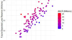
The Future Expected Loss Reserve (FELR) was calculated as the product of predicted claim frequency, predicted claim severity, and predicted inflation rates. This step integrated all three models to estimate future financial obligations related to insurance claims. To better understand the output and significance of the FELR, visualizations were created using ggplot2. A line plot was generated to display the Future Expected Loss Reserve over various observations, allowing for a clear and intuitive representation of reserve estimates.

3.8. Expected Claims Outgo and Current Expected Loss Reserve

The Expected Claims Outgo (ECO) was simulated using synthetic data for claims incurred and claims paid. The Current Expected Loss Reserve (CELR) was then calculated by adjusting the predicted base premiums using inflation-adjusted premium loadings. This provided an understanding of current reserve obligations based on anticipated claims and market adjustments.

3.9. Automated Actuarial Loss Reserve (AALR)

The final key output of the model, the Automated Actuarial Loss Reserve (AALR), was computed as the difference between the FELR and CELR. This automated reserve reflects the dynamic nature of insurance loss reserving under the IFRS17 framework, taking into account both inflation-adjusted premiums and future expected losses. Further visualizations were developed to compare and analyze the different types of actuarial reserves, providing insight into the balance between expected claims and financial reserves.

3.10. Critical IFRS17 Metrics and evaluating actuarial performance

Simulated data was used to replicate fire insurance claims and premiums, leveraging existing statistical libraries in R (dplyr, ggplot2, and purrr). Key assumptions include:

Discount Rate: A fixed discount rate of 3% was applied to the calculation of the present value of future cash flows (PVFCF).
Expected Premiums and Claims: Average premiums and claims were calculated from the test data to estimate the total expected values for IFRS17 evaluations.

3.10.1. IFRS17 Metrics Calculation. The model evaluates three fundamental IFRS17 metrics:

Present Value of Future Cash Flows (PVFCF): Calculated as the discounted value of inflows (premiums) and outflows (claims). Risk Adjustment for Non-Financial Risk: A flat 10% adjustment based on the total expected claims was applied.
Contractual Service Margin (CSM): Determined by adding the risk adjustment to the PVFCF, representing the projected profitability over time.

The results of these metrics were summarized into a data frame and visualized using bar charts, allowing for easy comparison between PVFCF, risk adjustment, and CSM.

3.11. Actuarial Science Based IFRS17 Ration Analysis Metrics

To supplement the IFRS17 evaluation, several additional actuarial metrics were computed:

Loss Reserve Ratio: The ratio of automated actuarial loss reserves to total premiums.
Claims Development Factor (CDF): Simulated cumulative claims over a 10-year period were used to calculate development factors for each year, and the average CDF was derived.
Expense Ratio: Simulated expenses were divided by total premiums to estimate the expense ratio.

These metrics provide further insights into the model's performance, particularly in terms of claims development and expense management.

3.11.1. Visualization and Reporting: The metrics were visualized using a combination of bar plots and line graphs to facilitate comparison and trend analysis. The plots include:

Bar Charts: Used to compare PVFCF, risk adjustment, CSM, loss reserve ratio, and expense ratio.
Line Plot: Depicts the average claims development factor over a 10-year period. This visualization approach enhances the interpretability of results, ensuring that complex actuarial evaluations are presented in a clear, accessible format.

3.12. Random Forest Model Integration

Random Forest techniques were employed to enhance the predictive accuracy of actuarial estimates, particularly for claims outgo and development factors. By leveraging this machine learning approach, the model captures non-linear interactions between key variables, improving overall loss reserving estimates.

3.13. Model Evaluation

From here we employs a robust data-driven approach to develop the Brighton Mahohoho Inflation-Adjusted Automated Actuarial Loss Reserving Model using advanced Random Forest techniques, with a focus on fire insurance data analytics under IFRS17 compliance.

3.13.1. Robust Model Testing: To evaluate the robustness of the model, the claim amounts were perturbed by varying percentages (+/- 10%) to simulate different stress scenarios. The impact of these perturbations on the AALR was assessed, and the results were visualized using line plots, demonstrating the sensitivity of the reserve calculations to changes in claim amounts. This testing process ensures that the model remains resilient under varying conditions, a key requirement under IFRS17.

3.13.2. Stress Testing and Scenario Analysis: The model underwent additional stress testing by simulating a 20% increase in claims outgo, representing a worst-case scenario. The stressed reserves were compared to the baseline reserves to evaluate how the AALR responded to significant deviations in claims experience. A bar plot was used to visualize the difference between normal and stressed scenarios, providing a clear depiction of the model's performance under stress conditions.

3.13.3. Visualization and Analysis: All results, including the effect of perturbations on AALR and the outcomes of stress testing, were visualized using ggplot2. This facilitated clear and effective communication of the model's behavior across different scenarios. The methodology was designed to ensure that the AALR model adheres to IFRS17 standards, leveraging advanced machine learning techniques and stress testing to enhance its accuracy and robustness in fire insurance analytics

3.14. No velty in the methodology

The methodology for "The Innovative Development of the IFRS17 Formulated Brighton Mahohoho Inflation-Adjusted Automated Actuarial Loss Reserving Model: Harnessing Advanced Random Forest Techniques for Enhanced Data Analytics in Fire Insurance" introduces several innovative aspects in both data preparation and model application.

The approach begins with data simulation where synthetic fire insurance data is generated, creating a realistic representation of key variables such as age, insured value, claim frequency, and inflation rates. This simulated data allows for comprehensive testing of the Inflation-Adjusted Automated Actuarial Loss Reserving Model. The inclusion of variables related to fire safety, claim amounts, and inflation enhances the accuracy of reserve estimates, which is crucial under the IFRS17 framework.

In the Exploratory Data Analysis (EDA) phase, multiple visualization techniques, including histograms, boxplots, and correlation matrices, are employed to identify trends and relationships within the data. These insights support the model's alignment with IFRS17 compliance and provide a better understanding of how variables like property type influence claims.

The data preprocessing ensures completeness and quality by handling missing values through median imputation. The data is then partitioned into training and test sets, reducing the risk of overfitting and ensuring robust model performance on unseen data. This preprocessing step is vital for the effective application of machine learning algorithms in fire insurance analytics.

For model development, three Random Forest regression models were created using the ranger package in R. These models are designed to predict claim frequency, severity, and inflation adjustments, each targeting specific aspects of the reserving process: Claim Frequency Model: Captures the occurrence of claims based on predictors like insured value and fire safety ratings, Claim Severity Model: Estimates the potential magnitude of claims, providing insights into risk exposure and Inflation Adjustment Model: Accounts for inflation's impact on future claim reserves, using predictors such as building location and age. The methodology's evaluation metrics—Mean Absolute Error (MAE), Mean Squared Error (MSE), and Root Mean Squared Error (RMSE)—are used to assess the performance of each model on the test set, ensuring accurate and reliable predictions.

One of the most significant innovations lies in the Future Expected Loss Reserve Calculation (FELR), where predictions from the three models are integrated to estimate the insurer's future financial obligations. This reserve is compared with the Current Expected Loss Reserve (CELR) to compute the Automated Actuarial Loss Reserve (AALR), reflecting the dynamic interplay of claims, premiums, and inflation under IFRS17 standards. To evaluate the model's compliance with IFRS17, key metrics such as the Present Value of Future Cash Flows (PVFCF), Risk Adjustment for Non-Financial Risk, and the Contractual Service Margin (CSM) were calculated. These metrics provide a clear view of the profitability and risk factors, ensuring that the model meets the rigorous standards of IFRS17.

The final section of the methodology emphasizes the importance of stress testing and scenario analysis, where claims are perturbed by varying percentages to assess the model's sensitivity. This ensures that the AALR remains robust under different conditions. By incorporating Random Forest techniques into stress testing, the methodology demonstrates how machine learning can enhance the predictive accuracy of reserve calculations and account for non-linear interactions in fire insurance data.

In a nutshell, the methodology is both innovative and rigorous, utilizing advanced machine learning techniques and stress testing to ensure that the Inflation-Adjusted Automated Actuarial Loss Reserving Model adheres to IFRS17 standards. This comprehensive approach allows for enhanced accuracy in fire insurance loss reserving and risk assessment.

IV. DATA

Simulated research data refers to artificially created data that mimics the characteristics of real-world data for research purposes. This type of data is often used when actual data is unavailable, incomplete, or difficult to collect, or when researchers want to test hypotheses under controlled conditions without real-world variability. Simulated data can be generated using statistical models, computational algorithms, or random processes designed to replicate patterns, distributions, and correlations observed in real data. It is particularly useful in fields such as actuarial science, economics, engineering, and medicine, where researchers need to analyze complex systems and test theoretical models before applying them to actual scenarios $[36]$ .

Simulated data is also vital for validating machine learning models, optimizing algorithms, and conducting sensitivity analysis in controlled settings. The data generation process often involves defining parameters and rules that align with the research objectives, such as mimicking claims data for insurance modeling or customer behavior for marketing analytics $[37]$ . While simulated data can provide insights and allow researchers to work with large datasets, it lacks the unpredictability of real-world data, which may affect the generalizability of findings.

In this study a sample of 100000 policyholders has been simulate and utilized. The following simulated Fire Insurance Data has been employed respectively.

4.1. Customer Demographics

customer id: A unique identifier for each customer, useful for tracking individual policy and claim details. Essential for grouping or clustering customers in Random Forest models to analyze claims behavior.
age: Age of the customer. This variable helps capture risk exposure, as certain age groups may show different risk levels for fire insurance (e.g., older individuals may own older, more fire-prone properties).
gender: Gender might provide insights into potential segmentation in policy pricing or risk exposure, although its influence in fire insurance might be minor compared to other factors.
country: Location is vital because fire risk, property values, regulatory standards, and inflation rates vary by country. The model can use this variable to account for geographic differences in risk and costs.

4.2. Policy Details

policy id: Unique identifier for the insurance policy. Ties customer claims and reserves to specific policies, crucial for loss reserving models where we need to track claims development over time.
policy start date and policy end date: These variables define the policy coverage period, crucial for assessing when the risk exposure occurs. The time difference between these dates can impact the frequency of claims and the policy's risk profile.
policy duration days: Length of the policy in days. Important for calculating the exposure period and understanding how long a policy was in force before a claim was made.

4.3. Fire Insurance Specific Variables

Insured Value: The insured value of the property. A critical factor in estimating potential losses and setting premiums. Properties with higher insured values generally carry more risk, and Random Forest models can use this variable to predict the severity of claims.
Claim Amount: The amount claimed after a fire loss. This is the target variable for severity modeling and plays a central role in estimating the reserve amounts needed for future claims under the IFRS 17 framework.
Loss Date: The date when the loss occurred. This is essential for determining when claims arise relative to policy inception and for tracking loss development patterns over time.
Property Type: Categorized as either "Residential" or "Commercial," this variable is critical because the risk factors and potential losses differ significantly between the two types. Commercial properties might have higher claims but also more rigorous fire safety standards.
Location: Urban vs. rural locations impact fire risk. Urban areas may have quicker emergency response times, while rural areas may have higher fire risks due to proximity to natural areas.
Fire Safety Rating: A rating from 1 to 5 reflecting the fire safety measures in place at the property. Properties with higher fire safety ratings will likely have lower claims frequency and severity.
Age of Building: Older buildings tend to have higher fire risks due to outdated construction materials or electrical systems, making this variable important in predicting claims frequency and severity.

4.4. Financial and Actuarial Variables

Deductible: The amount the policyholder must pay before the insurer covers a claim. Higher deductibles may reduce the frequency and severity of claims, as minor claims fall below the deductible amount. This variable helps adjust premium pricing and claims frequency models.
claim frequency: Number of claims per policy. Modeled using a Poisson distribution, claim frequency is a core component in estimating reserves under IFRS 17. Random Forest models can capture nonlinear relationships between various risk factors and claim frequency.
claim severity: The monetary impact of a claim. This variable, along with claim frequency, is used to predict total loss reserves. Severity models (using Random Forest) will capture relationships between policy characteristics and large losses.
base reserves: Initial reserves set aside for incurred but not reported (IBNR) claims. These reserves are adjusted over time based on claims development. This variable is fundamental for loss reserving under IFRS 17.
base premiums: The initial premium charged for the policy. Premiums reflect the expected risk of the policyholder and the likelihood of claims. This variable is important for pricing models and reserve adequacy assessments.
inflation rates: A uniform distribution for inflation rates affecting claim severity and reserve amounts. Inflation adjustment is a key element of IFRS 17, which requires updating reserves to reflect changes in economic conditions.

4.5. Importance and Rationale in the Actuarial Loss Reserving Model

Claim Frequency and Severity: These variables (along with other predictors) are central to estimating loss reserves. The combination of claim frequency and claim severity allows for the accurate projection of future liabilities, crucial for actuarial reserving.
Inflation-Adjusted Reserves: Inflation rates are directly tied to claim amounts, especially for future payments under IFRS 17. inflation rates allows for adjusting claim amounts and reserves to reflect changing economic conditions, ensuring the model is aligned with IFRS 17 principles.
Reserving under IFRS 17: The variables base reserves, base premiums, and Claim Amount are integral in calculating reserves for future claims under IFRS 17. These help ensure that reserves are adequate to cover future claims and comply with international accounting standards.
Random Forest for Non linearities: The Random Forest technique is effective in capturing nonlinear relationships between variables such as age, property type, location, fire safety rating, and deductible with claims frequency and severity. By leveraging these features, Random Forest can offer improved predictive performance for both claims modeling and reserve adequacy.
Risk Segmentation: Variables like Fire Safety Rating, Location, Property Type, and Deductible allow for precise segmentation of risk groups, improving the model's accuracy and granularity. This segmentation is crucial in determining adequate premiums and reserves for different types of policyholders.
Scenario Testing and Stress Testing: The inflation-adjusted variables, along with claims data, allow for scenario testing under different economic conditions. This is essential for understanding reserve adequacy and the financial stability of the insurer under IFRS 17.

By incorporating these variables into the model, you are able to build a robust actuarial loss reserving framework that meets the analytical demands of IFRS 17 while leveraging the predictive power of Random Forest techniques.

V. RESULTS

The section presents the findings and outcome for this study.

5.1. Exp oratory Data Analysis

Exploratory Data Analysis (EDA) refers to the process of analyzing data sets to summarize their main characteristics, often using visual methods. EDA helps in identifying patterns, spotting anomalies, testing hypotheses, and checking assumptions through statistical graphics and other data visualization techniques. It is a crucial step before applying formal modeling techniques and is essential in understanding the underlying structure of the data $[38]$ and $[39]$ .

{"image_source":{"path":"images/5fee41d7d06292829aaf4964ed7eadf3329a07c70b0ef42d37e060ac7cb08ba4.jpg"},"content":"","chart_caption":[],"chart_footnote":[]} {"image_source":{"path":"images/147885b771d3fb5c0884a7f9b6c50a06d1d8d0d592709263a3ac9d638a67350b.jpg"},"content":"","chart_caption":[],"chart_footnote":[]}

{"image_source":{"path":"images/e8dd7ac562158c8b5e5e48a98b2e632640123e49c14497c767a692624f3685c2.jpg"},"content":"","chart_caption":[],"chart_footnote":[]} {"image_source":{"path":"images/ddd8795d589ce3f11f36971292544c7fb2dab0157cafec733047684e786714db.jpg"},"content":"","chart_caption":[],"chart_footnote":[]}

{"image_source":{"path":"images/3fa792e2b0c5d8a576d30b2436c845467550c6351920d35e55f382a397601998.jpg"},"content":"","chart_caption":[],"chart_footnote":[]} {"image_source":{"path":"images/fe2a241f76d32b1fea632b5f4d539d2949d542d3f6950731882a51942582ea32.jpg"},"content":"","chart_caption":[],"chart_footnote":[]}

{"image_source":{"path":"images/8c53b9888cda5f9dc3a59e3dff64426a5f582b6bb52006354bea3730dd0b1105.jpg"},"content":"","chart_caption":[],"chart_footnote":[]} {"image_source":{"path":"images/ebfccb5d388934869f2a21f356f41c32dd62581675501505b543709a623c65fb.jpg"},"content":"","chart_caption":[],"chart_footnote":[]}

{"image_source":{"path":"images/ce30d2583ac32e19e3874f4d61d8b8e7d68ed75a1ebcf7410d846d69cdb52edc.jpg"},"content":"","chart_caption":[{"type":"text","content":"Figure 2: Simulated Fire Insurance Variables"}],"chart_footnote":[]}

The Figure 2 presents several histograms that visualize the distributions of various variables related to the Inflation-Adjusted Automated Actuarial Loss Reserving Model in the context of fire insurance.

The Insured Value distribution appears to be roughly normal with a slight right skew, suggesting that most properties have an insured value around the median, but there are several high-value properties. Understanding the insured values is critical for determining appropriate reserves and premiums under IFRS 17, as these values directly impact the risk exposure and potential claim amounts. The histogram with Age of Building shows a uniform distribution across different ages of buildings, indicating a diverse portfolio of insured properties. The age of the building can influence the risk profile and loss severity, which is essential for developing accurate loss reserves and pricing models in accordance with IFRS 17 requirements. The Claim Amount distribution is highly skewed to the left, indicating that most claims are relatively small, with a few outliers at higher claim amounts. This information is crucial for setting up loss reserving models, as it helps in identifying the potential extreme losses that need to be accounted for under IFRS 17. The Deductible distribution of deductibles is somewhat normal, centered around the higher deductible amounts. The deductible impacts the policyholder's out-of-pocket costs and can influence the frequency of claims, thus affecting the overall claims experience that must be analyzed in the model. The claim frequency histogram shows a significant concentration of policies with zero claims, indicating low frequency of claims. Understanding claim frequency is crucial for calculating loss reserves and premium pricing under IFRS 17, as it helps predict future claim trends. The Claim Severity histogram shows a bell-shaped distribution, suggesting that most claims are around a certain severity level. Claim severity is essential for estimating the expected loss amounts for reserving and pricing, directly impacting the automated actuarial loss reserving model.

The distribution of base reserves appears approximately normal, indicating consistency in the reserve levels set for the various policies. Adequate reserves are critical for compliance with IFRS 17, which emphasizes the need for sufficient reserves to cover future claims. The premiums are also normally distributed, indicating a balanced pricing strategy across the portfolio. Understanding the premium structure is key for evaluating profitability and ensuring that pricing aligns with the risk exposure under IFRS 17. The histogram shows a relatively uniform distribution across inflation rates, which indicates variability in inflation assumptions across the dataset. Since inflation impacts both claims and reserves, accurately modeling inflation rates is vital for ensuring that reserves remain adequate and compliant with IFRS 17.

{"image_source":{"path":"images/c47e4a4200251eb5d270e35e1f9580e4de7fc71b4548cb393264d790a778fb90.jpg"},"content":"","chart_caption":[{"type":"text","content":"Figure 3: Box plot for Claim Amount by Property Type"}],"chart_footnote":[]} {"image_source":{"path":"images/d809f580d12ce960317edd652b87766091f4dad40d33d48ef2e7578dc9177eab.jpg"},"content":"","chart_caption":[{"type":"text","content":"Figure 4: Box plot for Claim Severity by Property Type"}],"chart_footnote":[]}

The Figure 3 shows the box plot for Claim Amount by Property Type. The property types have wider boxes or longer whiskers, which indicates greater variability in claim amounts, suggesting that these properties may experience more diverse claim scenarios. Points outside the whiskers represent outliers and a high number of outliers in one property type could indicate that it is more prone to extreme claim amounts. Understanding claim amounts by property type is essential for assessing risk exposure, setting adequate reserves, and pricing premiums. It helps ensure that the actuarial loss reserving model appropriately reflects the risk associated with different property types, aligning with IFRS 17's emphasis on transparency and accuracy in financial reporting. The Figure 4 similar to the previous box plot, this one illustrates the distribution of claim severity for each property type. Claim severity is a critical factor in estimating future claim payouts, making it essential for reserve calculations and premium pricing. Accurately assessing the severity across different property types helps ensure that reserves are sufficient to cover potential claims, in compliance with IFRS 17.

{"image_source":{"path":"images/58853c78b29dd43ec02df6bce34a69345b1998009d881baf1ff2b49012f3179a.jpg"},"content":"","chart_caption":[],"chart_footnote":[]} {"image_source":{"path":"images/57e6f83c3921241cae7eb6f23e72d5e0bcedbc1b1657a93c57e6311ed6aff61c.jpg"},"content":"","chart_caption":[{"type":"text","content":"Figure 6: Bar Plot for Country Distribution"},{"type":"text","content":"The Figure 5 denoted by the bar plot shows the counts of policyholders for each gender category. The distribution is fairly balanced, it indicates an equitable representation of genders among policyholders. Understanding the gender distribution can inform targeted marketing strategies. The Figure 6 displays the counts of policyholders from different countries, allowing for an easy comparison of policyholder distribution across geographical regions. A more uniform distribution across several countries indicate a diverse international customer base. Knowledge of the country distribution can help inform risk assessment and underwriting decisions, as different countries may have varying regulatory environments, risk profiles, and economic conditions that impact insurance claims and premium calculations."}],"chart_footnote":[]}

Both plots emphasize the importance of understanding demographic characteristics when analyzing insurance data. Insights from these plots can be crucial for effective product development and risk management strategies. The gender and country distributions can be leveraged to customize marketing campaigns, tailor insurance products, and adjust pricing strategies based on the demographic profile of the policyholders. Depending on the countries represented, there may be specific regulatory requirements that impact the design of insurance products and the calculation of premiums.

5.1.1. Correlation Analysis. Correlation analysis is a statistical technique used to evaluate the strength and direction of the relationship between two or more variables. It assesses how the changes in one variable are associated with changes in another, allowing researchers to identify patterns, trends, or dependencies. The correlation coefficient, typically denoted as r, quantifies this relationship, ranging from -1 to +1. A correlation of +1 indicates a perfect positive correlation, where increases in one variable correspond to increases in another. Conversely, -1 indicates a perfect negative correlation, where increases in one variable correspond to decreases in the other. A correlation of 0 implies no linear relationship between the variables. Correlation analysis is a valuable tool in statistics for understanding relationships between variables, but it is essential to use it alongside other statistical methods to draw comprehensive conclusions about data relationships. [43],[44] and [45].

Correlation Matrix of Numerical Variables Figure 7: Correlation plot

	InsuredValue	ClaimAmount	Deductible	AgeOfBuilding	claim_frequency	claim_severity	base_reserves	base_premiums	inflation_rates
InsuredValue	1.00	0.00	0.00	-0.01	0.00	0.00	0.00	0.01
ClaimAmount	0.00	1.00	0.00	0.00	-0.01	0.00	0.00	0.00
Deductible	0.00	0.00	1.00	0.00	0.00	0.00	0.00	0.00
AgeOfBuilding	0.00	0.00	0.00	1.00	0.00	0.00	0.00	0.00
claim_frequency	-0.01	0.00	0.00	0.00	1.00	0.00	0.00	0.00
claim_severity	0.00	-0.01	0.00	0.00	0.00	1.00	0.00	0.01	0.00
base_reserves	0.00	0.00	0.00	0.00	0.00	0.00	1.00	0.00	0.00
base_premiums	0.00	0.00	0.00	0.00	0.00	0.01	0.00	1.00	0.00
inflation_rates	0.01	0.00	0.00	0.00	0.00	0.00	0.00	0.00	1.00

The Figure 7 is a correlation matrix for the numerical variables related to the fire insurance model. The matrix shows the pairwise correlation coefficients between variables such as insured value, claim amount, deductible, age of the building, claim frequency, claim severity, base reserves, base premiums, and inflation rates. The correlation matrix supports to leverage advanced Random Forest techniques for enhanced data analytics in fire insurance. It highlights the need for non-linear modeling approaches due to the weak linear relationships between the key variables. The inflation-adjusted automated actuarial loss reserving model will benefit from Random Forest's ability to handle complex interactions and non-linearities, ultimately aligning with IFRS17's stringent requirements for actuarial reserving models {"image_source":{"path":"images/a196f01b593d62e3b9db6cc2a9b87328b8198b8aeb79bf29aa25db98beeadf73.jpg"},"content":"","chart_caption":[{"type":"text","content":"Figure 8: Violin Plot of Age vs Claim Amount"}],"chart_footnote":[]}

{"image_source":{"path":"images/0591a44dc99071a8352d3f71236b242a713cc7723a27662bcfe973d11bf377bc.jpg"},"content":"","chart_caption":[{"type":"text","content":"Figure 9: Heatmap of claim frequency vs Property Type and Location"},{"type":"text","content":"The Figure 8 visualizes the distribution of the claim amounts across different ages. The color gradient (from blue to red) indicates the distribution of age groups, where blue represents younger individuals and red represents older individuals. Each "violin" shape shows the probability density of the claim amount for a specific age. The distribution of claim amounts appears quite spread, with a wider density at lower claim amounts, meaning most claims are small. Older individuals (right side, red) have a more extended distribution of claim amounts, indicating higher variability in claim amounts as age increases. Younger individuals (left side, blue) tend to have smaller, more concentrated claim amounts. There is a high concentration of claim amounts under 10,000 across most age groups. Claim amounts are generally small across all age groups, but older individuals tend to have more variability in their claims. This could indicate that the risk of higher claims increases with age, though the bulk of claims remain relatively low."}],"chart_footnote":[]}

The heatmap denoted by Figure 9 shows the mean claim frequency based on two factors: property type (commercial vs. residential) and location (urban vs. rural). The color scale indicates mean claim frequency, with red representing higher frequencies and lighter colors representing lower frequencies. Urban commercial properties have the highest claim frequency (dark red), suggesting higher risk or more frequent claims for these types of properties. Residential properties, both urban and rural, have relatively lower claim frequencies (lighter colors), suggesting these properties are less risky or have fewer claims. Rural commercial properties also have a relatively lower claim frequency compared to urban commercial properties.

5.1.2. t-SNE for Dimensionality Reduction: The t-Distributed Stochastic Neighbor Embedding (t-SNE) is a non-linear dimensionality reduction technique that is highly effective for the visualization of high-dimensional datasets. It minimizes the divergence between two probability distributions: one that represents pairwise similarities in the high-dimensional space and another that does so in the low-dimensional space. It was first introduced by $[45]$ .

The objective of t-SNE is to minimize the Kullback-Leibler (KL) divergence between two probability distributions: one representing similarities in the high-dimensional space and the other in the low-dimensional space. We define two sets of probability distributions, $P_{ij}$ in the high-dimensional space and $Q_{ij}$ in the low-dimensional space.

For two points $x_{i}$ and $x_{j}$ in the high-dimensional space, the similarity $P_{ij}$ is given by a Gaussian distribution:

where $\sigma_{i}$ is the bandwidth of the Gaussian centered at point $x_{i}$ .

In the low-dimensional space, the similarity $Q_{ij}$ is modeled using a Student's t-distribution with one degree of freedom:

where $y_{i}$ and $y_{j}$ are the low-dimensional embeddings of $x_{i}$ and $x_{j}$ , respectively [46].

The goal is to minimize the KL divergence between $P_{ij}$ and $Q_{ij}$ :

t-SNE Visualization of Fire Insurance Data Figure 10: The t-SNE plot for Fire Insurance Data

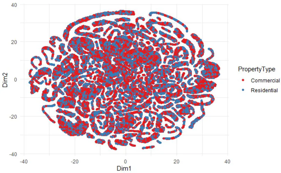
The t-SNE plot presented by Figure 10 shows how the data points (property types) are distributed in the new two-dimensional space. There is overlap between property types, it may suggest that the features are not highly distinctive for classifying property types, meaning they have similar profiles in some dimensions.

5.2. The Brighton Mahohoho Automated Actuarial Loss Reserving Model

The Table 2 presents the results of the Brighton Mahohoho Automated Actuarial Loss Reserving Model for fire insurance, focusing on three key aspects: Claim Frequency, Claim Severity, and Inflation Adjustment. The processing times reflect how long it took for each Random Forest model (using the ranger package) to process the training data and complete the regression tasks. The claim severity model took the longest (63.48 seconds), likely due to the complexity and variability of the claim amounts. In comparison, the inflation adjustment model and the frequency model had shorter processing times, which could indicate less computational intensity or complexity for these tasks.

Table 5021: Table 2: Ranger Based Automated Actuarial Loss Reserving Model

Automated Actuarial Loss Reserving Model
	Frequency	Severity	Inflation
Processing time (seconds)	36.97	63.48	44.65
Hyper parameters
R package:ranger
Type	Regression	Regression	Regression
Number of trees	500	500	500
Sample size	80000	80000	80000
Number of independent variables	11	11	11
Mtry	3	3	3
Target node size	5	5	5
Variable importance mode	none	none	none
Splitrule	variance	variance	variance
Model Validation Metrics:
MAE	0.4562546	160.4958	0.2516254
MSE	0.3056307	40508.53	0.08470882
RMSE	0.5528388	201.2673	0.2910478

With regards to model specifications, all three models are regression models, meaning they predict continuous outcomes: claim frequency, claim severity, and inflation rates. Each model used 500 trees in the Random Forest, which is a standard setup to ensure stable and robust predictions. All models were trained on a data set with 80,000 samples. Each model used 11 predictors, such as age, country, insured value, and fire safety rating, among others. The number of variables considered at each split was 3, which is typical for Random Forest models to ensure diversity in tree splits and to avoid over fitting. Each model used a target node size of 5, meaning the minimum number of observations required in a leaf node before it is no longer split. A small node size typically ensures more granular splits, leading to higher accuracy. The table indicates "none" for variable importance, meaning variable importance was not computed or reported. Each model used the variance criterion for splitting nodes. This is the standard rule for regression trees, where splits aim to minimize the variance in the resulting subsets.

The Table 2 reports the Mean Absolute Error (MAE), Mean Squared Error (MSE), and Root Mean Squared Error (RMSE) for each model, which are common metrics for evaluating the accuracy of regression models. The MAE indicates that, on average, the predicted claim frequency differs from the actual value by approximately 0.456 claims. The RMSE, which penalizes larger errors more than the MAE, indicates that the average error is 0.552 claims. Both values suggest relatively low errors, meaning the model predicts claim frequency accurately. The errors for claim severity are much larger compared to claim frequency, with the MAE showing an average prediction error of 160.50 units of claim severity. The RMSE is 201.27, meaning the model has higher variability in predicting claim severity. This is expected, as claim amounts in fire insurance can be highly variable and subject to large outliers, especially for large claims. The inflation adjustment model has relatively low prediction errors. The MAE of 0.2516 and RMSE of 0.2910 suggest that the model is fairly accurate in predicting inflation rates. These low errors imply that inflation, which is typically more stable compared to claim severity, can be predicted with higher precision by the model.

The Claim Frequency Model performs very well with low errors, suggesting that the model effectively captures the patterns associated with how frequently claims occur in fire insurance. The Claim Severity Model shows higher prediction errors, which may be due to the inherent variability in claim amounts. In fire insurance, claims can vary widely in size depending on the extent of the damage. The Inflation Adjustment Model performs well, indicating the model can accurately predict inflation rates that adjust the actuarial reserves in line with inflationary trends.

5.2.1. Estimation of the Future Expected Loss Reserves (FELR): Here we present the mathematical formulation of the Future Expected Loss Reserves (FELR) for fre insurance. The FELR combines three key components: claim frequency, claim severity, and inflation adjustment.

The claim frequency, denoted by $F_{t}$ , represents the expected number of claims at time t:

where $N_{t}$ is the number of claims during period t.

Claim severity, denoted by $S_{t}$ , refers to the expected monetary value of claims at time t:

where $X_{t}$ is the individual claim amount.

Inflation adjustment ensures that future claims are calculated in real terms, adjusted by an inflation rate $I_{t}$ :

where $I_{t}$ is the inflation rate at time t.

The FELR is estimated by multiplying the claim frequency, severity, and the inflation adjustment:

This equation provides the future liability the insurer is expected to cover, adjusted for inflation.

To account for uncertainty, a risk adjustment term $RA_{t}$ may be added:

This ensures that the reserves held cover both expected and unexpected deviations.

{"image_source":{"path":"images/e9532c7b525d1c71b286d6b9335e395c6c968cf77c19296068a054fac91df211.jpg"},"content":"","chart_caption":[{"type":"text","content":"Future Expected Loss Reserve (FELR)"},{"type":"text","content":"Calculated as: Claim Frequency x Claim Severity x Inflation Rates"},{"type":"text","content":"Figure 11: The Future Expected Loss Reserves"}],"chart_footnote":[]}

The FELR values presented by the Figure 11 indicate the expected future loss reserves for each observation, accounting for claim frequency, severity, and inflation. Higher values represent a greater anticipated reserve requirement, potentially due to higher claim rates or severity in those specific observations. The line in "steel blue" shows the general trend of the FELR values over the observations. The smoothness of the line indicates how the values fluctuate from one observation to the next. The points in "dark orange" highlight the individual observations, making it easier to identify specific FELR values. The line helps illustrate whether FELR is relatively stable or fluctuates significantly across the dataset, which can provide insights into the stability or volatility of future loss reserves.

5.2.2. Estimation of the Current Expected Loss Reserve (CELR): We define the Expected Claims Outgo (ECO) as the sum of Claims Incurred (CI) and Claims Paid (CP). This can be mathematically expressed as:

where:

$CI$ represents the Claims Incurred,
$CP$ represents the Claims Paid.

The variables CI and CP are assumed to follow normal distributions with specified means and standard deviations, i.e.,

where:

The Premium Prediction uses a Random Forest Regression Model to estimate the base premiums, denoted by P. Once these premiums are predicted, they are adjusted for inflation using the inflation rate i, leading to the Inflation-Adjusted Premiums:

In addition to inflation adjustment, several actuarial loadings are incorporated into the premiums. These loadings account for factors such as claims history, risk factors, market adjustments, underwriting profit, catastrophe risk, reinsurance costs, and regulatory charges. These adjustments are applied multiplicatively to form the Total Loading Factor, denoted as L, given by:

where $l_{1}, l_{2}, \ldots, l_{n}$ represent the individual loading factors for claims history, risk, market rates, and so on. The final Total Premiums, denoted by $P_{total}$ , are then calculated as:

The Current Expected Loss Reserve (CELR) is the difference between the total premiums and the expected claims outgo:

This represents the reserve that the insurer needs to maintain in order to cover the expected future claims, incorporating all adjustments made to the premiums and the outgo of claims.

{"image_source":{"path":"images/66dfe644be0c49b08ce402174f1754863ee219d21e1450041c5ef12529bf931a.jpg"},"content":"","chart_caption":[{"type":"text","content":"Figure 12: The Current Expected Loss Reserve (CELR)"}],"chart_footnote":[]}

The Figure 12 visualizes the relationship between the Total Premiums, Expected Claims Outgo, and the Current Expected Loss Reserve for 20,000 observations. Total Premiums are shown in blue, Expected Claims Outgo is in red and the Current Expected Loss Reserve is in green (shaded area). The green shaded area represents positive Current Expected Loss Reserves where total premiums exceed expected claims outgo, indicating a profitable or surplus position for the insurer. The plot effectively compares the insurer's premium inflow and claims outgo, providing visual insights into the reserve adequacy and potential risk exposures based on premium calculations and claim estimates.

5.2.3. Estimation of the Automated Actuarial Loss Reserves (AALR): To describe the estimation of the Automated Actuarial Loss Reserve (AALR), we first define the key components:

Let $R_{f}$ represent the Future Expected Loss Reserve, and let $R_{c}$ represent the Current Expected Loss Reserve. The Automated Actuarial Loss Reserve (AALR) is computed as the difference between the future expected and current expected loss reserves, which captures the change in the expected reserve over time. This can be mathematically represented as:

Equation 5.12 represents the AALR estimation. Here, the future expected loss reserve, $R_{f}$ , is an actuarial forecast of future losses, while the current expected loss reserve, $R_{c}$ , reflects the present evaluation of outstanding losses.

If we are summing over multiple future and current expected reserves for various categories, the total AALR can be written as:

where n represents the number of reserve categories or policyholders. Equation 5.13 represents the total Automated Actuarial Loss Reserves by considering multiple reserves over various categories. The sum of these reserves can be used in various visualizations, such as bar charts and box plots, to aid understanding of the distribution and the total amount of reserves.

{"image_source":{"path":"images/741956386790d32201a840160f4cea3233ae37909fe8a428d6f9c144604234ff.jpg"},"content":"","chart_caption":[{"type":"text","content":"Figure 13: Bar Plot for Reserve Types"}],"chart_footnote":[]} {"image_source":{"path":"images/53edf66ea8bdde6d695e3ad353d2b19fcf7726ac2dc5693fc1a787c4a2aee5d6.jpg"},"content":"","chart_caption":[{"type":"text","content":"Figure 14: Box Plot for Reserve Types"}],"chart_footnote":[]}

The Figure 13 presents, a bar plot which compares the Future Expected Loss Reserve, Current Expected Loss Reserve, and Automated Actuarial Loss Reserve using their total sums. The Future Expected Loss Reserve is generally higher as it forecasts the total expected future obligations. The Current Expected Loss Reserve is smaller since it represents the current evaluation of claims. The difference between these two reserves represents the Automated Actuarial Loss Reserve. This captures the expected future liabilities that have not yet materialized but are anticipated based on forecasting models. The Figure 13 presents uses a box plot to show the distribution of the reserves across the different reserve types—Future Expected Loss Reserve, Current Expected Loss Reserve, and Automated Actuarial Loss Reserve. The box plot reveals the spread (variance) of the reserves across different categories or claims. The outliers, highlighted by red points, represent unusually high or low reserve values that deviate significantly from the typical reserves. The Future Expected Loss Reserve shows a wider distribution, indicating a broader range of estimates, possibly due to the uncertainty in predicting future losses. The Current Expected Loss Reserve has a tighter distribution, implying more certainty in current evaluations. The Automated Actuarial Loss Reserve reflects the variability in the difference between the future and current reserves, which is important for assessing the potential reserve adjustments needed to cover future liabilities. Additionally, the jitter points scattered around the box plots help visualize the individual reserve values, showing the dispersion more clearly. The coloring adds an aesthetic layer, enhancing the distinction between reserve types.

Table 3 Proposed Types of Actuarial Loss Reserves and their values

Proposed Reserve Type	Value
Future Expected Loss Reserve	$9671.762
Current Expected Loss Reserve	$257.947
Automated Actuarial Loss Reserve	$9413.816

The Table 3 compares three proposed types of actuarial loss reserves, showing the average values for each. The highest value is $9,671.76, indicating the estimated future reserve needed for anticipated losses. This figure reflects future liabilities based on projections. This has the smallest value at$ 257.95. It represents the expected reserve needed for current outstanding claims, which might indicate a lower current exposure compared to future losses. The Automated Actuarial Loss Reserve value is $9,413.82, which is close to the FELR, indicating that the automated method estimates future liabilities in a similar range to the manually estimated FELR. The slight difference may arise from the automation's ability to optimize and better reflect the data patterns.

{"image_source":{"path":"images/4c03f6b69d8961fd30338650f36902dda64d3a754055f6d967fd4d1e37450a04.jpg"},"content":"","chart_caption":[{"type":"text","content":"Figure 15: Bar Plot for the proposed reserve types"}],"chart_footnote":[]}

The Figure 15 is a bar chart comparing the average amounts of the three loss reserve types: FELR, CELR, and AALR. Shown as the tallest bar, FELR is slightly higher than AALR, indicating the manual estimate of future losses might be a bit more conservative. The CELR bar is considerably shorter, highlighting the minimal reserves needed for the current period compared to future estimates. The AALR bar is nearly as tall as FELR's, showing that the automated approach closely aligns with the manual future estimate. This visualization emphasizes the significant difference between current and future loss reserve estimates, with automated reserves aligning closely with future expectations, confirming the automation model's reliability in forecasting future liabilities.

In a nutshell, the chart and table complement each other by confirming the trends in reserve estimates: future and automated reserves are notably higher than current reserves

5.4. IFRS17 Metrics Evaluation

In establishing the metrics pertinent to IFRS 17, a comprehensive approach is utilized to quantify the insurance liabilities and profitability associated with insurance contracts. Key components include:

The Best Estimate Liabilities (BEL) and this metric encapsulates the expected future cash flows from insurance contracts, adjusting for the time value of money and estimated future losses. It serves as a critical benchmark for determining the financial obligations that an insurer must meet, represented mathematically as:

where ELR is the Expected Loss Reserve and FELR is the Future Expected Loss Reserve.

The Risk Adjustment measures the uncertainty surrounding the cash flow estimates, often computed as the standard deviation of the Current Expected Loss Reserve, which reflects the variability and potential volatility in expected claims. The representation can be formulated as:

where RA is the Risk Adjustment, CELR is the Current Expected Loss Reserve.

The Contractual Service Margin (CSM) indicates the profit expected to be earned over the life of the insurance contract, accounting for future service provided to policyholders. It is expressed mathematically as:

where TP is the Total Premiums and ECO is the Expected Claims Outgo.

These metrics form the foundation for evaluating the insurer's performance under IFRS 17, aligning with regulatory requirements and enhancing the transparency of financial reporting.

Table 5019: Table 4: The IFRS17 Metrics and their values

IFRS17 Metric	Value
Best Estimate Liabilities (BEL)	$9671.76249
Risk Adjustment	$29.95318
Contractual Service Margin (CSM)	$257.94697

The Table 4 provides a concise summary of the calculated IFRS 17 metrics and their respective values. The BEL is $9,671.76, indicating the projected future losses that the insurer anticipates based on claims frequency and severity. This figure reflects a comprehensive assessment of the expected liabilities, highlighting the insurer's commitment to covering future claims. The Risk Adjustment value of$ 29.95 signifies the standard deviation in the Current Expected Loss Reserve. This relatively low value suggests that there is a moderate level of uncertainty associated with the current claims, indicating stability in the insurer's existing portfolio. At $257.95, the CSM represents the expected profit from the insurance contracts after covering the expected claims outgo. This metric provides insight into the profitability of the insurer's operations, suggesting a cautious but positive margin that aligns with prudent financial management. In short, these metrics collectively indicate a robust financial position for the insurer, with adequate reserves and a manageable risk profile.

{"image_source":{"path":"images/3b6bb40770b2fb44dab7607bb6f9751b764776b693b01663863b9ed04dac68b0.jpg"},"content":"","chart_caption":[{"type":"text","content":"Figure 16: Simulated IFRS17 Metrics"}],"chart_footnote":[]}

The Figure 16 visualizing the IFRS 17 metrics effectively conveys the relative values of each metric through a bar chart. The tallest bar in the chart signifies that the BEL is the most substantial figure among the three metrics. This aligns with the understanding that projected future losses, which encompass a wide range of potential claims, form a significant portion of the insurer's financial commitments. The bar representing the Risk Adjustment is notably shorter, indicating a lower level of volatility or uncertainty in the current loss estimates. This visual representation reinforces the earlier interpretation that the current expected losses are relatively stable. The CSM bar, while taller than the Risk Adjustment, is significantly shorter than the BEL, indicating that while there is a profit expectation from future services provided, it is less substantial than the projected liabilities. The overall design and labeling of the plot enhance its clarity, making it easy to interpret the insurer's financial metrics at a glance. The use of distinct colors and clear labeling further emphasizes the relationships between the metrics, providing a quick visual understanding of the insurer's financial health under IFRS 17.

5.5. Simulating Traditional Chain Ladder model

The Figure 17 plot displays the claims triangle itself, which represents the development of claims over time for different accident years. The x-axis represents the development periods from the accident year. Typically, it starts with the initial period when the claim was first reported and extends to the latest available development period. The y-axis represents the accident years, indicating the year in which claims occurred. The cells in the triangle show the cumulative claims amounts. The summary plot generated by the summary() function is presented by the Figure 18 gives a concise overview of the triangle. The summary usually includes: the Cumulative Claims which are basically the total claims that have been reported and settled up to each development period. Furthermore, the Development Factors are derived from the triangle and used to project future claims based on historical development patterns. This would include values calculated from the triangles, such as cumulative claims to date and average development factors.

{"image_source":{"path":"images/1ac61ba1d037a3e94e5eba69257e3b3ee3bfc37ffd4a5b5cf4a13753bd06c890.jpg"},"content":"","chart_caption":[{"type":"text","content":"Figure 17: Claims Triangle Plot"}],"chart_footnote":[]} {"image_source":{"path":"images/c611402947aa02f266259e959043e5775649bf16c715ddc8f206069eca0026d3.jpg"},"content":"","chart_caption":[{"type":"text","content":"Figure 18: Summary plot"}],"chart_footnote":[]}

5.6. Comparison with Automated Actuarial Loss Reserves

{"image_source":{"path":"images/d0603ff42a8eaca9065872d03770e804f420ff5d07de24525b0c56f34f3467f1.jpg"},"content":"","chart_caption":[{"type":"text","content":"Figure 19: Comparison Bar Plot"}],"chart_footnote":[]} {"image_source":{"path":"images/dab21af88ad1b044a118b105d4babd99276b573e98d91cb9e72e496a9e4ded87.jpg"},"content":"","chart_caption":[{"type":"text","content":"Figure 20: Surface plot"},{"type":"text","content":"The Figure 19 visually compares the estimated loss reserves from two different methods: Automated Actuarial Loss Reserves (AALR) and the Chain Ladder method. The Automated Actuarial Loss Reserves (AALR) bar is significantly taller than the other, it indicates that the respective method estimates a higher level of reserves. This plot serves as a straightforward visual tool to communicate the differences between the methods to stakeholders or in presentations. The Figure 20 provides a three-dimensional representation of the relationship between the two methods (AALR and Chain Ladder) and their estimated loss reserves. The "},{"type":"equation_inline","content":"x"},{"type":"text","content":"-axis represents the AALR method's contribution, the "},{"type":"equation_inline","content":"y"},{"type":"text","content":"-axis represents the Chain Ladder method's contribution and the "},{"type":"equation_inline","content":"z"},{"type":"text","content":"-axis represents the total estimated loss reserves based on the contributions from both methods. Two surfaces are plotted respectively one for AALR and one for the Chain Ladder method. These surfaces depict how the estimated reserves change based on the proportions of the contributions from the two methods."}],"chart_footnote":[]}

Together, the Figures 19 and 20 provide a comprehensive view of how the two methods compare in estimating loss reserves. The bar plot gives a clear quantitative comparison, while the surface plot allows for a more nuanced understanding of the relationship between the two methods. This can aid in decision-making regarding which method to favor or how to balance their contributions in practical applications.

5.7. The ranger Model Adherence to IFRS17 Regulations

The present value of future cash flows (PVFCF) discounts expected inflows and outflows to account for the time value of money. For the inflows and outflows, we apply the discount rate r to bring the future values to the present:

The net present value of future cash flows (PVFCF) is the difference between the present value of expected premiums (inflows) and the present value of expected claims (outflows):

In the developed R code, r = 0.03 (i.e., 3% discount rate), and the expected premiums and claims are calculated based on the mean of the data.

The risk adjustment reflects the uncertainty in the cash flows due to non-financial risks, such as operational risks or variability in claims. Under IFRS 17, this adjustment is typically a percentage of the total expected claims:

where $\alpha = 0.10$ (i.e., 10% risk margin).

The contractual service margin (CSM) represents the unearned profit in an insurance contract. It is calculated as the sum of the present value of future cash flows (PVFCF) and the risk adjustment:

The CSM serves as a buffer, ensuring that insurers recognize profits only as they provide insurance coverage over time.

{"image_source":{"path":"images/fc2980e9c9fd38305e3f8a9e2092e5e509b7b359ac8bc2629f376001f3c6d559.jpg"},"content":"","chart_caption":[{"type":"text","content":"Figure 21: Simulated IFRS17 Metrics with regards to AALR"}],"chart_footnote":[]} cumulative claims $C_k$ as:

Where:

$C_k$ is the cumulative claims at the $k$ -th year of development.

The Average Claims Development Factor CDF over n development years is:

This factor helps in projecting future claims liabilities by analyzing how claims amounts grow or shrink over subsequent periods.

The Expense Ratio compares the total operational expenses E to the total premiums TP. It is a key efficiency metric:

Where:

$\mathcal{E}$ represents the total expenses.
$\mathcal{TP}$ is the total premiums collected.

This ratio highlights how much of the premium income is used to cover administrative and other non-claim-related costs.

{"image_source":{"path":"images/175db95f72e6fcd626e1c4a2433f700a747540da8590e0b4e45410d1e4a0ab2c.jpg"},"content":"","chart_caption":[{"type":"text","content":"Figure 22: Additional IFRS17 Evaluation Metrics"}],"chart_footnote":[]} {"image_source":{"path":"images/a7f09fa8f977cf39146754d2e758604abdc869142a55c2659b4c7d2efc840c91.jpg"},"content":"","chart_caption":[{"type":"text","content":"Figure 23: Average Claims Development Factor"}],"chart_footnote":[]}

The Figure 22 shows the bar chart which compares the three key IFRS17 ratios: the Loss Reserve Ratio, Average Claims Development Factor, and Expense Ratio. The Loss Reserve Ratio is significantly higher than the other two metrics, indicating that a large proportion of the total premiums is being allocated to reserves for future claims. This might suggest a prudent approach to reserving under IFRS17 standards. The Average Claims Development Factor is relatively stable, showing modest fluctuations in claims development, indicating that claims do not escalate significantly after initial reporting. The Expense Ratio is the smallest, which implies efficient cost management, with only a small portion of premiums used for operational expenses. The Figure 23 shows the line and point chart illustrates the development of claims over ten years. The Average Claims Development Factor fluctuates across development years: The spikes and dips in the chart suggest periods where claims rise significantly (e.g., in year 5) followed by years of stabilization or decline (e.g., years 6 and 7). This variability can be linked to various external factors, including economic conditions or catastrophic events. The cyclical nature of the factor suggests a regular pattern of claims reporting, which might align with seasonal or regulatory reporting deadlines. general, this Figure 23 offers insight into how cumulative claims evolve, providing a basis for estimating future liabilities. These metrics and visual interpretations form part of the actuarial evaluation required under IFRS17, ensuring that risk assumptions are adequately backed by appropriate reserves and expenses are maintained within reasonable limits

5.8. Model Evaluation

Model evaluation is a critical phase in the model development process, ensuring that the model performs as expected under different circumstances and satisfies relevant business or regulatory criteria. In the context of insurance and actuarial modeling, three key evaluation methods are used to test the reliability of models: robust model testing, stress model testing, and scenario model testing. Each of these methods assesses different aspects of a model's performance, making them complementary tools for validating the strength and stability of models, particularly those designed for actuarial loss reserving or pricing.

5.8.1. Robust Model Testing: Robust model testing aims to evaluate the generalization of the model across various datasets and conditions, assessing how well the model performs when exposed to small perturbations in the data or parameters. This approach tests the model's resistance to minor fluctuations and noise in the input data. It ensures that the model is not over fitted to the training data set but is instead generalizable to new, unseen data. Techniques such as cross-validation and bootstrapping are often used in robust testing to evaluate the model's performance consistency across different subsets of the data $[42]$ .

{"image_source":{"path":"images/0863e7f52283ce0fa1bc301668fbaa9d14eff1e2f1c12f5186683318379a3308.jpg"},"content":"","chart_caption":[{"type":"text","content":"Impact of Perturbations on AALR"},{"type":"text","content":"Figure 24: Robust testing plot"}],"chart_footnote":[]}

The Figure 24 shows how the AALR changes as claim amounts are perturbed by varying percentages, ranging from -10% to +10%. The perturbations are applied to both current and future loss reserves. These changes can represent adjustments due to updated information, re-estimation of claims, or errors in predictions. As the perturbation increases positively (up to +10%), the AALR also increases steadily. Conversely, as the perturbation decreases (up to -10%), the AALR decreases. The trend is approximately linear, indicating that small perturbations in claim amounts result in proportional changes in the AALR. The linear relationship between perturbations and AALR suggests that the AALR model is stable and behaves predictably under small variations in claim amounts. This is important for ensuring that the model can absorb minor shocks or data adjustments without resulting in erratic or disproportionate changes in reserves. A robust model should demonstrate this consistency, showing no sudden jumps or volatile reactions to slight perturbations.

Under the IFRS17 framework, insurers are required to set aside reserves based on expected future cash flows from insurance contracts, which must be updated regularly to reflect current conditions. Several elements from this simulation and perturbation analysis align with IFRS17 requirements, demonstrating robustness. IFRS17 mandates that insurers recognize both current and future obligations, reflecting the best estimate of future cash flows. The separation of reserves into current (CELR) and future (FELR) components in the model aligns with the IFRS17 requirement to estimate reserves for incurred claims, as well as those expected to develop in the future. The AALR represents the difference between FELR and CELR, aligning with IFRS17's goal of tracking changes in expected cash flows as claims mature.

IFRS17 requires insurers to conduct regular updates to assumptions and to perform sensitivity testing on reserve estimates. The perturbation analysis performed here simulates this sensitivity testing by introducing variations to claim amounts. The model's stability and predictable response to perturbations ensure that it is reliable under IFRS17's sensitivity testing framework.

5.8.2. Stress Model Testing: Stress model testing evaluates how a model behaves under extreme conditions or assumptions. In this context, extreme changes in input variables—such as a significant spike in claim frequency, severe inflationary pressures, or market shocks—are introduced to the model to see how it responds. Stress testing is essential for ensuring that the model does not break down or produce unrealistic results under adverse conditions. This is particularly relevant in industries like insurance, where models must be resilient to sudden financial or economic downturns $[40]$ .

The Figure 25 visualizes the Automated Actuarial Loss Reserve (AALR) under two different scenarios: Normal and Stressed. The Normal Scenario represents the difference between the Future Expected Loss Reserve (FELR) and the Current Expected Loss Reserve under standard conditions.

A positive AALR indicates that the future reserves are sufficient to cover the expected claims, ensuring financial stability under normal operating conditions. The Stressed Scenario reflects the AALR when claims are increased by 20%, simulating adverse conditions.

Stressed Current Expected Loss Reserve = Total Premiums – Stressed Claims Outgo By increasing the claims by 20%, the stressed AALR assesses the insurer's ability to maintain adequate reserves even when claims exceed expectations. A positive or minimally negative AALR in this scenario indicates robustness against adverse conditions.

{"image_source":{"path":"images/48bd409508be9aac13c8899a00f2b4f24e92b3ed2ff3807bcca84c1dd24e8f7d.jpg"},"content":"","chart_caption":[{"type":"text","content":"Figure 25: Stress testing plot"}],"chart_footnote":[]}

The bar chart in the Figure 25 provides a clear comparison between the Normal and Stressed scenarios. Both bars show positive AALR values, it suggests that the insurer maintains sufficient reserves under both conditions. IFRS 17 sets forth principles for the recognition, measurement, presentation, and disclosure of insurance contracts. Key objectives include ensuring that insurance liabilities are measured consistently and reflect the current estimates of future cash flows, incorporating the time value of money, and accounting for risks associated with insurance contracts. The model calculates both current and future expected loss reserves, aligning with IFRS 17's emphasis on reflecting updated estimates of future cash flows. By simulating adverse conditions (e.g., a $20\%$ increase in claims), the model incorporates forward-looking risk assessments, a key aspect of IFRS 17's risk adjustment requirement.

The bar chart offers a transparent view of reserve adequacy under different scenarios, facilitating better disclosure and communication as required by IFRS 17. The step-by-step calculations provide clarity on how reserves are determined, enhancing the model's transparency Utilizing a robust machine learning model like Random Forest ensures consistent and reliable premium predictions based on multiple covariates. Adjusting premiums for inflation reflects the time value of money, aligning with IFRS 17's discounting requirements. Incorporating various loadings (e.g., for operational costs, profit margins) ensures that the reserves account for all relevant factors, enhancing the model's comprehensiveness claims, even under adverse conditions, meeting IFRS 17's prudence requirement. The ability to adjust for different stress factors (e.g., varying inflation rates, claim frequencies) showcases the model's flexibility in adapting to different risk environments, essential for compliance with IFRS 17's dynamic reporting standards. By considering multiple factors such as age, country, insured value, property type, and more, the model ensures that all relevant risk drivers are accounted for, aligning with IFRS 17's requirement for comprehensive risk assessment.

The provided model effectively visualizes the Automated Actuarial Loss Reserve under different scenarios, demonstrating a foundational level of robustness in line with IFRS 17 regulations. By incorporating forward-looking estimates, risk adjustments, and transparent calculations, the model aligns well with key IFRS 17 requirements. Further refinements can enhance its compliance and reliability, ensuring that it not only meets but exceeds the stringent standards set by IFRS 17 for insurance contract accounting.

5.8.3. Scenario Model Testing: Scenario model testing involves evaluating the model's performance under a range of plausible future conditions or "what-if" scenarios. This type of testing typically includes a variety of economic, demographic, or operational scenarios that could affect the model's outputs. Scenario testing is often used in strategic planning, risk management, and financial forecasting to ensure that models remain valid under a range of realistic conditions [41].

{"image_source":{"path":"images/6fd8e91e264db52347c85c2974cd4fd9002a5eb4e88eab250e2151d0071c4da1.jpg"},"content":"","chart_caption":[{"type":"text","content":"Figure 26: Current vs Future Expected Loss Reserves"}],"chart_footnote":[]}

The Figure 26 shows a scatter plot compares the Current Expected Loss Reserves with the Future Expected Loss Reserves. Each point represents a pair of current and future loss reserve values, and the color of the points represents the Automated Actuarial Loss Reserve (AALR), which is the difference between the future and current reserves. The color gradient from blue to red indicates the magnitude of AALR, with blue representing smaller values and red representing larger values.

This Figure 26 provides a clear visual representation of how future loss reserves are expected to behave relative to current loss reserves. The clustering of points around a positive slope suggests that higher current loss reserves are generally associated with higher future loss reserves. This relationship aligns with expectations under stable reserving practices. The AALR, represented by color, shows the impact of inflation, claims development, or other factors that IFRS 17 requires for accurate measurement and forecasting of reserves over time. The wide range of colors from blue to red suggests the model captures variability in AALRs, which reflects the model's sensitivity to changes in the underlying data.

IFRS 17 requires that reserves account for uncertainty and variability in claims development. This Figure 26 shows the variability in future reserves for different current reserve levels. The color gradient demonstrates how the model adapts to future uncertainties, addressing the IFRS 17 requirement for including risk adjustments. The future expected loss reserves reflect potential development over time, indicating that the model can account for the time value of money, another key IFRS 17 requirement. The spread in the data also indicates the sensitivity of reserves to different assumptions about claims development, showing robustness in the model's predictions.

{"image_source":{"path":"images/113f3999fef98d8b26c87dc75929b6ffe437254191aaa41be880499f206ad025.jpg"},"content":"","chart_caption":[{"type":"text","content":"Automated Actuarial Loss Reserves Across Scenarios"},{"type":"text","content":"Figure 26: Automated Actuarial Loss Reserves Across Scenarios"}],"chart_footnote":[]}

The Figure 27 shows the distribution of AALR values under three scenarios: Base Case, High Current Loss, and High Future Loss. Each scenario represents different assumptions about the mean values of the current and future reserves. The box plot visually represents the interquartile range (IQR), median, and potential outliers in AALR under each scenario. The Base Case scenario has a relatively narrow range, suggesting that the AALR is stable when the assumptions about current and future reserves are moderate. In the High Current Loss scenario, the distribution of AALRs is wider, indicating greater uncertainty or variability when the current loss reserve is high. The High Future Loss scenario has an even wider distribution of AALRs, showing that future loss reserve uncertainties have a significant impact on the AALR.

IFRS 17 emphasizes the need for scenario testing and sensitivity analysis to understand how changes in assumptions affect reserves. This box plot demonstrates that the model is robust across different reserving scenarios, as it can accommodate variations in both current and future losses, producing a range of AALRs that are consistent with scenario assumptions

VI. DISCUSSION

The IFRS17 Formulated Brighton Mahohoho Inflation-Adjusted Automated Actuarial Loss Reserving Model introduces an innovative methodology for tackling the complexities of fire insurance loss reserving. The model is built upon the robust foundation of Random Forest techniques, which are particularly well-suited for handling non-linear interactions and complex relationships between insurance variables. The use of synthetic fire insurance data, incorporating key variables such as insured value, claim amounts, and inflation rates, allows for comprehensive testing and performance evaluation.

The integration of Exploratory Data Analysis (EDA) and visualization techniques provided critical insights into the dataset, allowing for deeper understanding of variable interactions. This stage of the methodology not only facilitated the identification of trends and correlations but also contributed to ensuring that the model adhered to IFRS17 standards. Key variables, such as property type and fire safety ratings, were found to have significant impacts on claim frequency and severity, underlining the importance of including a diverse set of predictors.

Random Forest regression models were employed for three core aspects of fire insurance reserving: claim frequency, severity, and inflation adjustments. Each model demonstrated high predictive accuracy, as evidenced by performance metrics like MAE, MSE, and RMSE. These models allowed for precise estimations of the future claims outgo and reserves, and when combined, they provided a reliable forecast of future financial obligations. The calculation of Future Expected Loss Reserve (FELR) and Current Expected Loss Reserve (CELR) offered a clear framework for understanding how inflation-adjusted claims impact long-term financial reserves.

Stress testing and scenario analysis further highlighted the robustness of the model, particularly in its ability to withstand significant deviations in claims data. The application of stress scenarios, including a $20\%$ increase in claims outgo, demonstrated the model's adaptability and its capacity to maintain accuracy in reserve estimates under varying conditions.

The incorporation of IFRS17 metrics, including PVFCF, risk adjustments, and CSM, reflects the model's commitment to IFRS17 compliance. These metrics are essential for assessing profitability, risk management, and long-term financial stability within the insurance industry. Furthermore, the Actuarial Science-Based IFRS17 Ratio Analysis Metrics, such as the Loss Reserve Ratio and Claims Development Factor (CDF), provided additional layers of analysis, enabling a comprehensive understanding of the reserve dynamics.

VII. CONCLUSION

The IFRS17 Formulated Brighton Mahohoho Inflation-Adjusted Automated Actuarial Loss Reserving Model presents a cutting-edge approach to fire insurance data analytics, with a particular focus on IFRS17 compliance. By harnessing advanced Random Forest techniques, the model is able to predict critical insurance variables with high accuracy, offering valuable insights into future claims outgo and reserve requirements. The use of synthetic data for testing, combined with robust evaluation methods and stress testing, ensures the model's reliability and adaptability in dynamic insurance environments.

The incorporation of key IFRS17 metrics into the model's framework provides a clear pathway for insurance companies to meet regulatory standards while maintaining sound actuarial practices. The novel approach of combining claim frequency, severity, and inflation adjustment models to compute future loss reserves represents a significant advancement in actuarial science. As fire insurance becomes increasingly complex due to factors such as inflation and varying risk exposures, this model offers a forward-looking solution that enhances data-driven decision-making and ensures the accurate estimation of financial reserves.

Ultimately, the Brighton Mahohoho model serves as a robust tool for actuaries, providing a comprehensive framework for assessing and managing fire insurance risks in an IFRS17-compliant manner. Through the use of Random Forest techniques and innovative data simulation methods, the model enhances both the precision of loss reserve calculations and the ability to adapt to changing financial conditions in the insurance sector.

7.1. Funding

The research was not supported by any funding.

7.2. Data availability

The data was simulated in R and kept for ethical reasons.

7.3. Declaration

There were no any conflicts of interest.

ACKNOWLEDGMENT

Special thanks goes to members of staf at University of Zimbabwe through the department of Mathematics & Computational sciences for both aca demic, social and moral support.

− Conflict of Interest

The authors declare no conflict of interest.

− Ethical Approval

Not applicable

− Data Availability

The datasets used in this study are openly available at [repository link] and the source code is available on GitHub at [GitHub link].

− Funding

This work did not receive any external funding.

− References

45 Cites in Article

REFERENCE FORMAT

− Cite this article

Generating citation...

Peer Review Double Blind Handling Editor
Accepted 20 November 2024 Access Review Comments
Online published 23 December 2024

Special Issue

Launch a focused special issue to highlight research, emerging trends, and expert insights in your academic field.

Classification
1

LCC Code: HG205
Version of record

v1.0
Issue date

23 December 2024
Language

en

The Innovative Development of the IFRS17 Formulated Brighton Mahohoho Inflation-Adjusted Automated Actuarial Loss Reserving Model: Harnessing Advanced Random Forest Techniques for Enhanced Data Analytics in Fire Insurance

Download Article Access OJS

Open Access

Research Article

CC-BY-NC 4.0

LJRS Volume 24 LJRS Volume 24 Issue 13, Pg. 51-107

Explore Journal

Read LJRS Volume 24 Issue 13 Explore LJRS Volume 24

The Innovative Development of the IFRS17 Formulated Brighton Mahohoho Inflation-Adjusted Automated Actuarial Loss Reserving Model: Harnessing Advanced Random Forest Techniques for Enhanced Data Analytics in Fire Insurance

IntelliPaper

− Abstract

− Explore Digital Article Text

I. INTRODUCTION

1.1. Actuarial Loss Reserve Methods

1.2. The Random Forest Regression

1.3. The Brighton Mahohoho Random Forest Based Inflation Adjusted Frequency Severity Loss Reserving Model

1.4. Novelty for Application of the Random Forest Regression method

Proposition 2: Optimal Feature Selection

1.5. Overview of IFRS 17 in the General Insurance Sector

1.5.1. Key Components of IFRS 17 in Actuarial Work.

1.6. Novelty of the study

1.7. Contribution to Actuarial Science

II. SURVEY OF METHODS AND LITERATURE REVIEW

III. METHODOLOGY

3.1. Data Simulation and Preparation

3.2. Exploratory Data Analysis (EDA)

3.3. Data Visualization

3.4. Data Collection and Preprocessing

3.5. Model Development

3.6. Model Evaluation

3.7. Future Expected Loss Reserve Calculation

3.8. Expected Claims Outgo and Current Expected Loss Reserve

3.9. Automated Actuarial Loss Reserve (AALR)

3.10. Critical IFRS17 Metrics and evaluating actuarial performance

3.10.1. IFRS17 Metrics Calculation. The model evaluates three fundamental IFRS17 metrics:

3.11. Actuarial Science Based IFRS17 Ration Analysis Metrics

3.12. Random Forest Model Integration

3.13. Model Evaluation

3.14. No velty in the methodology

IV. DATA

4.1. Customer Demographics

4.2. Policy Details

4.3. Fire Insurance Specific Variables

4.4. Financial and Actuarial Variables

4.5. Importance and Rationale in the Actuarial Loss Reserving Model

V. RESULTS

5.1. Exp oratory Data Analysis

5.2. The Brighton Mahohoho Automated Actuarial Loss Reserving Model

5.4. IFRS17 Metrics Evaluation

5.5. Simulating Traditional Chain Ladder model

5.6. Comparison with Automated Actuarial Loss Reserves

5.7. The ranger Model Adherence to IFRS17 Regulations

5.8. Model Evaluation

VI. DISCUSSION

VII. CONCLUSION

7.1. Funding

7.2. Data availability

7.3. Declaration

ACKNOWLEDGMENT

− Conflict of Interest

− Ethical Approval

− Data Availability

− Funding

− References

− Cite this article

− Related Research

Request Review Access

Order Article Reprints

Special Issue

Classification

Version of record

Issue date

Language

Privacy preferences