




IntelliPaper
Abstract
A two-stage (rough and accurate) computation strategy was developed in this study in order to accurately calculate the minimum one-sided Hausdorff distance between continuous plane curves under a similarity transformation. In the rough computation, a mathematical programming model based on the discretisation method was constructed to ascertain the minimum one-sided Hausdorff distance. In addition, the linearisation method in this model was elucidated. Based on that, the solutions were attained through a stable and efficient simplex method and 5 characteristic points were obtained. In the accurate computation, a local iterative accurate algorithm for computing the minimum one-sided Hausdorff distance was established after 4 similarity transformation parameters were separated from 10 curve parameters corresponding to 5 characteristic points. Similar results, which verify the feasibility of this algorithm, were obtained based on rough and accurate computations in a numerical example. Moreover, a roundness error evaluation programming model based on the minimum one-sided Hausdorff distance and relevant linear solution methods was also developed. Furthermore, the numerical examples based on this model were compared with those based on a conventional roundness error computation model. The results revealed that similar computation circle centre coordinates, roundness error, and characteristic points can be obtained based on both models. The computational efficiency can be significantly improved via the method proposed in this study.Continuous plane curve, Minimum one-sided Hausdorff distance, Exact algorithm, Comparison of computational efficiency, Roundness error evaluation.
Explore Digital Article Text
I. INTRODUCTION
Early Hausdorff distance computation is mainly applied to pattern recognition and image processing, including the recognition of faces, fingerprints, characters, handwriting, and licence plates. However, there has been little investigation into the computation of the Hausdorff distance relative to non-point sets. In the conventional method, continuous geometric objects are discretised into point sets, based on which the approximate Hausdorff distance between continuous geometric objects can be indirectly obtained by computing the Hausdorff distance between point sets. More recently the computation of the Hausdorff distance between continuous geometric objects has been studied owing to potential demands in geometric modelling, computational geometry, computer graphics, and other fields. In 2008, Alt et al. from Germany demonstrated four cases of the one-sided Hausdorff distance between two C continuous plane curves. Specifically, the Hausdorff distance may present at two endpoints of two curves, with one of the two-points being the end-point of one curve, double perpendicular foot points, or the intersection point of the midline of one curve and another curve. Furthermore, they provided nonlinear constraint simultaneous equations corresponding to the four cases. The Hausdorff distance between plane curves was computed with the aid of a standard algebraic equations solver. In the same year, Elber et al. from Israel generalised these four cases of the one-sided Hausdorff distance between two continuous plane curves to space curves/ curved surfaces. They obtained the corresponding Hausdorff distance using a self-designed algebraic equations solver. In 2010, Chen et al. tackled the lack of research in finding the root of nonlinear simultaneous equations in previous studies [1-2].
They explored the geometric clipping method for calculating the Hausdorff distance between two B-spline curves. As per their algorithm, sufficient conditions allowing the Hausdorff distance to appear at the end of a curve were provided. The curve segmentation technique and rolling circle clipping method were adopted to transform the Hausdorff distance computation between two curves into that of the minimum or maximum distance between points and curves, thus improving the stability and computational efficiency of the algorithm. In the same year, Kim et al. proposed a real-time algorithm to accurately calculate the Hausdorff distance between two plane free-form curves. Firstly, G continuous double circular arcs were employed to approximate the free-form curves under given tolerances. The arcs were subsequently subjected to distance mapping and saved to a graphics hardware depth buffer. Finally, most of the redundant arc segments were trimmed to improve the computational efficiency related to the Hausdorff distance. In 2011, Bai et al. proposed a polyline method to obtain the Hausdorff distance between plane curves. Based on the algorithm, continuous free-form curves were approximated with polylines under a given measurement. An incremental algorithm was subsequently utilised to compute the one-sided Hausdorff distance between line segments and polylines. Since two clipping strategies are used in this method, the ineffective line segments in the final Hausdorff distance computation are clipped which significantly improves the computational efficiency.
In terms of the computation of the minimum Hausdorff distance between geometric objects under a certain transformation, Huttenlocher proposed an algorithm to compute the minimum Hausdorff distance for one- and two-dimensional point sets. The one-dimensional algorithm of the minimum Hausdorff distance between point sets was applied to the comparison computation of planar polygons under an affine transformation by using the affine arc length to represent planar polygons. The two-dimensional algorithm was used to compare digital images. Additionally, the Hausdorff distance definition was extended to enable it to be used for the comparison between partial sets. In further studies, Huttenlocher improved the minimum Hausdorff distance algorithm under a translation transformation between point sets and line segment sets by using a Voronoi diagram. According to two given polygons, Alt proposed that the Hausdorff distance between two polygons can be minimised by the rigid transformation of one of the polygons, and therefore the approximate matching between polygons can be realised. Chew et al. investigated the computational complexity of the minimum Hausdorff distance algorithm between geometric objects under a rigid transformation for planar line segments that are composed of point sets and polygon sets that are composed of point sets. Hur et al. adopted the conic section represented by a quadratic rational Bezier curve to perform the best uniform approximation (BUA) for the convolution curve of two plane curves. The objective was to minimise the Hausdorff distance between the conic section and the convolution curve. Because the weight factor of the rational Bezier curve was the only optimisation variable in the approximation curve in the model, the study revealed that there were two characteristic points on the approximation curve, and both the distance between them and the convolution curve were the Hausdorff distance, and the derivative signs of the two distances with respect to the weight factor were opposite. This constituted the necessary and sufficient conditions for minimising the Hausdorff distance between two curves. An iterative algorithm was also formulated for computing the BUA based on the necessary and sufficient conditions.
To ensure equal precision and computational efficiency, Gu et al. proposed a rough and accurate staged matching method between plane curves under an affine transformation. Liang et al. designed a matching method between plane curves using their projection along any direction based on a weak perspective projection model. Gruen et al. established a similarity transformation model consisting of seven parameters between curved surfaces as per the least squares principle. In addition, they considered the matching method between curved surfaces and applied it to the automatic mosaic of 3D point cloud data. Rodriguez et al. analysed the similarity computation between 3D curves through the string edit distance method. Yamany et al. formulated a surface registration method based on a genetic algorithm. Cao et al. transformed the Hausdorff distance computation between plane curves into that of the minimum distance from points to curves. This method eliminated the drawback of traditional methods, whereby different nonlinear simultaneous equations had to be solved separately under four Hausdorff distance cases between plane curves. Moreover, they constructed an algorithm to compute the one-sided Hausdorff distance between C2 continuous curves via two steps, namely rough and accurate computations. Based on a previous study , Cao et al. established a programming model for the minimum one-sided Hausdorff distance between plane curves under a rigid transformation and developed relevant solutions. Furthermore, they applied the model to line profile error evaluation.
As suggested in relevant studies, the computation of the Hausdorff distance between continuous curves and curved surfaces has attracted the attention of researchers in geometric modelling, computational geometry, computer graphics, and other fields in recent years. However, it also prevents the wider application of the Hausdorff distance in engineering. There are several issues in relevant research work. 1) A few studies have been conducted on the computation of the Hausdorff distance between free-form curves and curved surfaces. In most cases, the Hausdorff distance was obtained by solving simultaneous algebraic equations. Since the solution of these algebraic equations was either regarded as a black box or obtained by a standard solver, the solutions with a reference value and geometric significance cannot be fully provided. 2) Due to the complexity of concrete curves and curved surfaces in engineering, research on the computation of the Hausdorff distance between continuous curves or curved surfaces and the minimum Hausdorff distance under a certain transformation is still in its infancy. At the same time the lack of relevant solution methods significantly hinders its extensive application in the engineering field.
In this study, a mathematical programming model for computing the minimum one-sided Hausdorff distance between plane curves under a similarity transformation was constructed based on a previous study by supplementing the scale transformation parameters of approximation objects. A solution strategy composed of two-stage (rough and accurate) computation was proposed for this model. Moreover, a local iterative accurate algorithm for computing the minimum one-sided Hausdorff distance for continuous curves was also constructed. On that basis, a roundness error evaluation programming model, based on the minimum one-sided Hausdorff distance, was established and then verified numerically.
II. COMPUTATION OF THE MINIMUM ONE-SIDED HAUSDORFF DISTANCE BETWEEN PLANE CURVES UNDER A SIMILARITY TRANSFORMATION
2.1 Mathematical Programming Model
It can be inferred from the definition of the one-sided Hausdorff distance that the computation of involves the shortest distance from a point a on Curve A to Curve B. As per geometric error evaluation theory and curve/curved surface approximation theory, this shortest distance is generally called an error. When Curve B is allowed to undergo a similarity transformation, its position and scale are transformed. The change in the parameter of the point on Curve B corresponding to the shortest distance from a point on Curve A to Curve B is termed parameter transformation. When the shortest distance from Point to the transformed Curve B is also transformed, it is termed error transformation. Therefore, the computation of under a similarity transformation incorporates position, scale, parameter, and error transformations.
The representation of Curve B under a similarity transformation is subsequently discussed. The similarity transformation of the given plane curve B includes three motions; namely translation, rotation, and scaling. The following homogeneous coordinates can be used to represent the translation matrix, rotation matrix, and scaling matrix, respectively, including
where, represents the translation coordinates along the X and Y axes; represents the rotation angle; represents the scaling rations in the X and Y directions; To maintain the shape of the graph unchanged before and after scaling, equal scaling would be adopted in the following discussion, namely . These parameters are collectively called the similarity transformation parameter X.
After the above three motions, the expression of Curve B can be obtained as:
where, X, Y denotes the coordinates of Curve B in Frame ; they are all functions of the curve parameter b.
From the perspective of the BUA of curves or curved surfaces, the one-sided Hausdorff distance between two geometric objects is the maximum deviation of the approximation object from the approximation target. Minimising the maximum deviation under some transformation is the optimisation objective of the BUA. The process of minimising the maximum deviation is characterised by saddle points and can therefore be explored by saddle point programming. Under a similarity transformation, if the scale and position parameters of the approximation object are taken as optimisation variables and the one-sided Hausdorff distance from the approximation object to the approximation target is minimised as the optimisation objective, the definition of the minimum one-sided Hausdorff distance can be expressed as the following mathematical programming form:
The first line in Equation (3) represents the objective function of the optimisation model and h is the characteristic parameter. The second line represents the optimisation model constraint function; namely that the characteristic parameter h shall be the one-sided Hausdorff distance between two curves under a certain set of transformation parameters represents the Euclidean distance between Point a on Curve A and Point b on Curve B under the transformation parameter X.
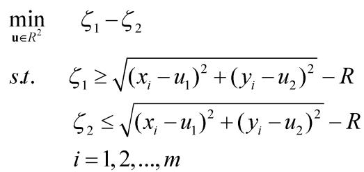
The constraint function in the above model is the one-sided Hausdorff distance between two curves under the transformation parameter . According to the definition of the one-sided Hausdorff distance between continuous curves in a previous study[16], it can be found that a pair of points satisfying the one-sided Hausdorff distance is the point pair satisfying the maximisation of the minimum distance and it also has the saddle point characteristics. Moreover, a saddle point programming model for the Hausdorff distance computation between two curves can be established if the curve parameters and of two curves are taken as optimisation variables and the minimum distance from a point on one curve to the other is taken as the optimisation objective. In other words, the computation of the minimum one-sided Hausdorff distance is an optimisation in Type min max min . To simplify the optimisation process, Curve A would be discretised to complete the computation of the shortest distance from each discrete point on Curve A to Curve B. On that basis, the following mathematical programming model can be constructed to obtain the solution to the minimum one-sided Hausdorff distance:
Following the discretisation of Curve A, the programming model given by Equation (3) can be expressed as:
where, represents the shortest distance from the discrete point on Curve A to the transformed curve , as presented in Figure 1. This can be computed according to the shortest distance algorithm from the point to the curve in a previous study ; represents the curve parameter corresponding to the minimum normal distance mapping point of the discrete point on Curve ; i represents the discrete point serial numbers, and m represents the total number of discrete points on Curve A. represents a similarity transformation parameter, and represents the optimisation variables of the saddle point programming model.
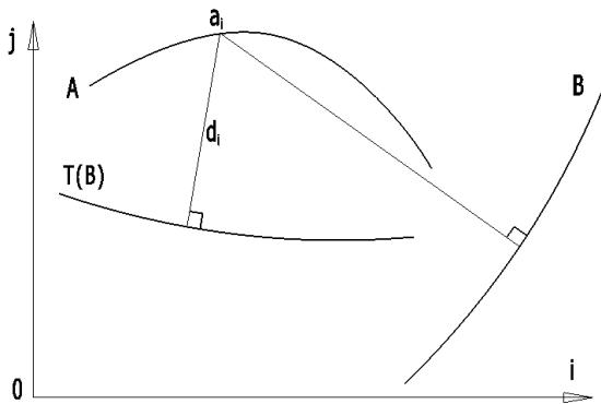 Fig. 1: Planar Curves under Similarity Transformation
It can be revealed from Equations (2) and (3) that the optimisation model constraint function given in Equation (4) is not a linear combination of optimisation variables, but a nonlinear optimisation which needs to be linearised.
2.2 Linearisation Solution to the Mathematical Programming Model
It can be seen from the above optimisation model that the nonlinear part of the optimisation variable is included in the shortest distance . If the shortest distance in Equation (4) is regarded as a function of the transformation parameter X, it can be expressed as follows:
If the transformation parameter is regarded as a first-order small quantity, it is called a small error. After in Equation (5) is subject to Taylor's expansion at the zero point of transformation parameters and their second-order and higher-order small quantities are omitted, the following expression can be obtained:
In the equation,
where, represents the shortest distance from a point on Curve A to Curve B before a similarity transformation; , and represent the first-order increment of the transformation parameter ; represents the coordinates of the point on Curve B; represents the coordinates of the unit normal vector at a point on Curve B; represents the first-order partial derivatives of Equation (2) for the transformation parameter .
After Equations (6) - (11) are substituted into Equation (4), the following linear programming model for computing the minimum one-sided Hausdorff distance between plane curves can be obtained:
where, h represents the characteristic parameter, that is, the one-sided Hausdorff distance from curve A to curve B; ; and m represents the number of discrete points on the actual curve.
The above optimisation model has the variable . However, are all free variables without non-negative requirements. To achieve the solutions by the simplex linear programming method, it can be arranged that and . Then, the slack variable ( ) is introduced and the inequality constraint is transformed into an equality constraint, finally an initial basic feasible solution can be obtained. Hence, the above linear programming problem can be expressed in the following standard form:
where, , represents a dimensional column vector of , represents a matrix of , and I represents an m-order unit matrix; , , and represent m-dimensional column vectors, and represents a 4-dimensional column vector; The upper corner mark T represents the matrix transposition.
After the above model is solved by the simplex linear programming method, the characteristic parameter h and the similarity transformation parameter of Curve B can be obtained. The value of the characteristic parameter can be considered as the minimum one-sided Hausdorff distance from curve A to curve B.
To reduce any error caused by the linear geometric model, curve B can be rotated, translated, and scaled, using the computation result of . The transformed curve can be regarded as a new curve and the above process can be repeated until the absolute value of the transformation parameters obtained from the computation of Equation (12) is less than the given precision.
Under the similarity transformation, one of the two curves (e.g., Curve B) can usually be translated, rotated, and scaled, so there are four degrees of freedom in Curve B. Therefore, when reaches its minimum, the equidistant line of Curve B has at least 5 points of tangency to Curve A, as shown in Figure 2. Under this condition, due to the continuous changes in the Curve B scale parameter s, when reaches the minimum, both the symmetric equidistant curves and of Curve B have points of tangency to Curve A. In other words, Curve A is bidirectionally enclosed by the inner and outer equidistant lines of Curve B and the maximum and minimum normal errors of Curve A relative to Curve B are equal in value and opposite in sign. The distribution ratio of the tangency points for the inner and outer equidistant curves and to Curve A can be 1:4 (4:1) or 2:3 (3:2).
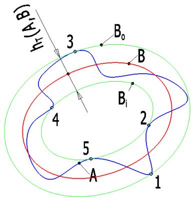 Fig. 2: Minimum one-sided HD from curve A to curve B where curve A is fixed and curve B subjects to the similarity transformation
2.3 Precise Iterative Model
The mathematical programming model in the previous section can be utilised to compute the minimum one-sided Hausdorff distance from discretised curve A to curve B. When the curve is originally provided in the form of discrete points, for example, when the curve is a data point obtained by measurement or the computational precision is not high, this method can meet the relevant requirements. However, when Curves A and B are presented as continuous curves, in order to obtain the precise minimum one-sided Hausdorff distance between both curves, it is necessary to conduct local iterative optimisations based on the previous section. Finally, the precise minimum one-sided Hausdorff distance from curve A to curve B can be obtained.
The approximate solution which satisfies the optimal condition can be obtained via the algorithm in the previous section. There are 5 characteristic points on discretised Curve A which are optimally arranged with the inner and outer equidistant lines of Curve B. It is necessary to construct a local iterative optimisation model, so that the parameters of Curves A and B, corresponding to 5 equivalent characteristic points, can meet the requirements of the one-sided Hausdorff distance.
As the local optimisation model contains 4 similarity transformation parameters and 10 curve parameters corresponding to 5 characteristic points, with a total of 14 optimisation variables, it can be considered a complex nonlinear problem. If these parameters can be solved together iteratively, the solution process is prone to oscillation, which may induce convergence failure in the computation. To reduce the computational difficulty and ensure computational stability, the precise iterative model is iteratively solved using two steps (similarity transformation parameters and curve parameters).
2.3.1 Similarity Transformation Parameter Iterative Solution
There are 5 initial points on Curve A and the mapping points with the shortest distance of on Curve B can be obtained by the algorithm of the shortest distance from points to curves. After the position of Point is fixed, the distance between corresponding can be equalised by changing the position, direction, and scale of Curve B. Therefore, the conditional expression can be provided:
where, the position of Point is related to the similarity transformation parameter of Curve B and its curve parameter b. Since Point is the normal mapping point with the shortest distance of on Curve B, its curve parameter is not independent, so . Hence, Equation (14) can be expressed as:
After Equation (15) is subject to Taylor's expansion near the initial point and the small quantity above the second order is omitted, the following expression can be obtained:
where, represents the function value of Function at the initial point; represents the first-order partial derivative of Function with respect to , respectively. Equation (16) can be represented in a matrix form and the following expression can be obtained:
The linear equations (17) can be solved to obtain the increments of similarity transformation parameters and these increments can be employed to update the Curve B similarity transformation parameters. Furthermore, the iterative process can be repeated until each similarity transformation parameter increment is smaller than the given computation precision .
2.3.2 Iterative Solution of Curve Parameters
When the minimum one-sided Hausdorff distance from curve A to curve B is achieved, the optimality condition and the one-sided Hausdorff distance condition are satisfied. The previous similarity transformation parameter iterative process ensured that the optimality conditions were satisfied. The condition satisfying the one-sided Hausdorff distance is discussed in this section. As reported in a previous study , the one-sided Hausdorff distance between plane curves is generally presented in four cases; double perpendicular foot points, one-to-two points, EA endpoints, and EB endpoints. Different constraint equations exist for different cases. The corresponding constraint equations are established according to the different situations of the 5 points on the actual Curve A before the iterative solution is performed. In this study, the one-sided Hausdorff distance between plane curves under the perpendicular foot point is selected as the example, and its corresponding conditions are:
Since the conditions of Equation (18) would definitely be satisfied, it is only necessary to locally optimise the parameters of Curve A at the characteristic point. After the Curve B similarity transformation parameters and the corresponding parameters of characteristic points on Curve B are set as initial points, the parameters of Curve A are the only undetermined variables in Equation (19). Hence, Equation (19) can be expressed as:
where, represents the curve parameter corresponding to the 5 characteristic points on Curve A.
Since the solution of Equation (20) is performed based on the previous programming algorithm and has a favourable initial point, the curve parameter increments corresponding to the 5 characteristic points on Curve A can be directly obtained by the efficient univariate Newton's iterative method. On that basis, each Curve A parameter can be updated and the iterative process can be repeated until the parameter increment is smaller than the given computation precision .
Due to the interaction between the iterative solution of the similarity transformation parameters and that of the curve parameters, it is necessary to conduct these two iterative processes alternately until the convergence conditions of the two iterative processes satisfy the requirements.
1.3 Numerical examples
The feasibility of the above algorithm is verified via numerical examples in this section. The original A and B curves are closed curves represented by the cubic uniform B spline, incorporating 90 control points. As shown in Figure 3, the red line represents Curve A and the blue line represents Curve B. Curve A is presented as an outline of a Liriodendron chinense leaf. The Curve B control points are obtained by superimposing an error function with a 2mm amplitude on 90 Curve A control points. Furthermore, the Curve B is transformed according to the following similarity transformation parameters: , , , and .
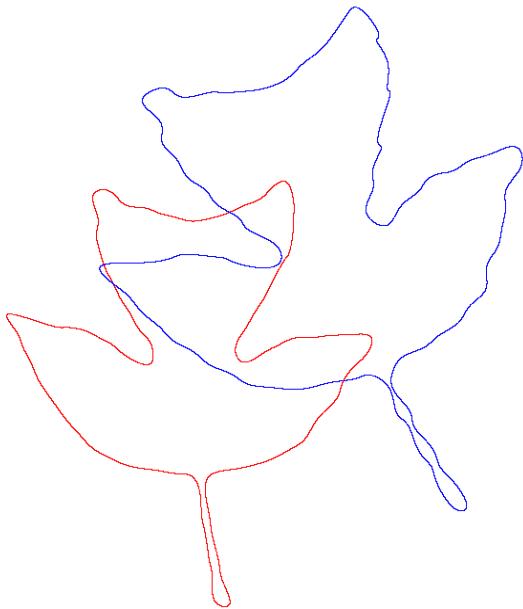 Fig. 3: The Original Curves A and B
The minimum one-sided Hausdorff distance from Curve A to Curve B can be calculated using the following process. Firstly, Curve A is discretised according to its parameters and Curve B is transformed from a B-spline form to a cubic piecewise Bezier curve through the algorithm in a previous study . Subsequently, the shortest distance from each discrete point on Curve A to Curve B is computed through the algorithm in a previous study , which can be regarded as the original normal error of Curve A relative to Curve B. The linear programming algorithm in Section 1.1 is then employed to compute the minimum one-sided Hausdorff distance from curve A to curve B under a similarity transformation. Subsequently, the corresponding transformation parameters, minimum one-sided Hausdorff distance , and corresponding characteristic point coordinates can be obtained. The computation precision is and the results are presented in Figure 4. The 5 pairs of blue points represent the corresponding characteristic points obtained by the mathematical programming method, and . The corresponding transformation parameters include , , , and . Based on the programming model computation results, can be solved precisely based on the local optimisation model in Section 1.2. The final characteristic points are presented as 5 pairs of red points in Figure 4, and , which is highly similar to the mathematical programming method results. The corresponding transformation parameters include , , , and .
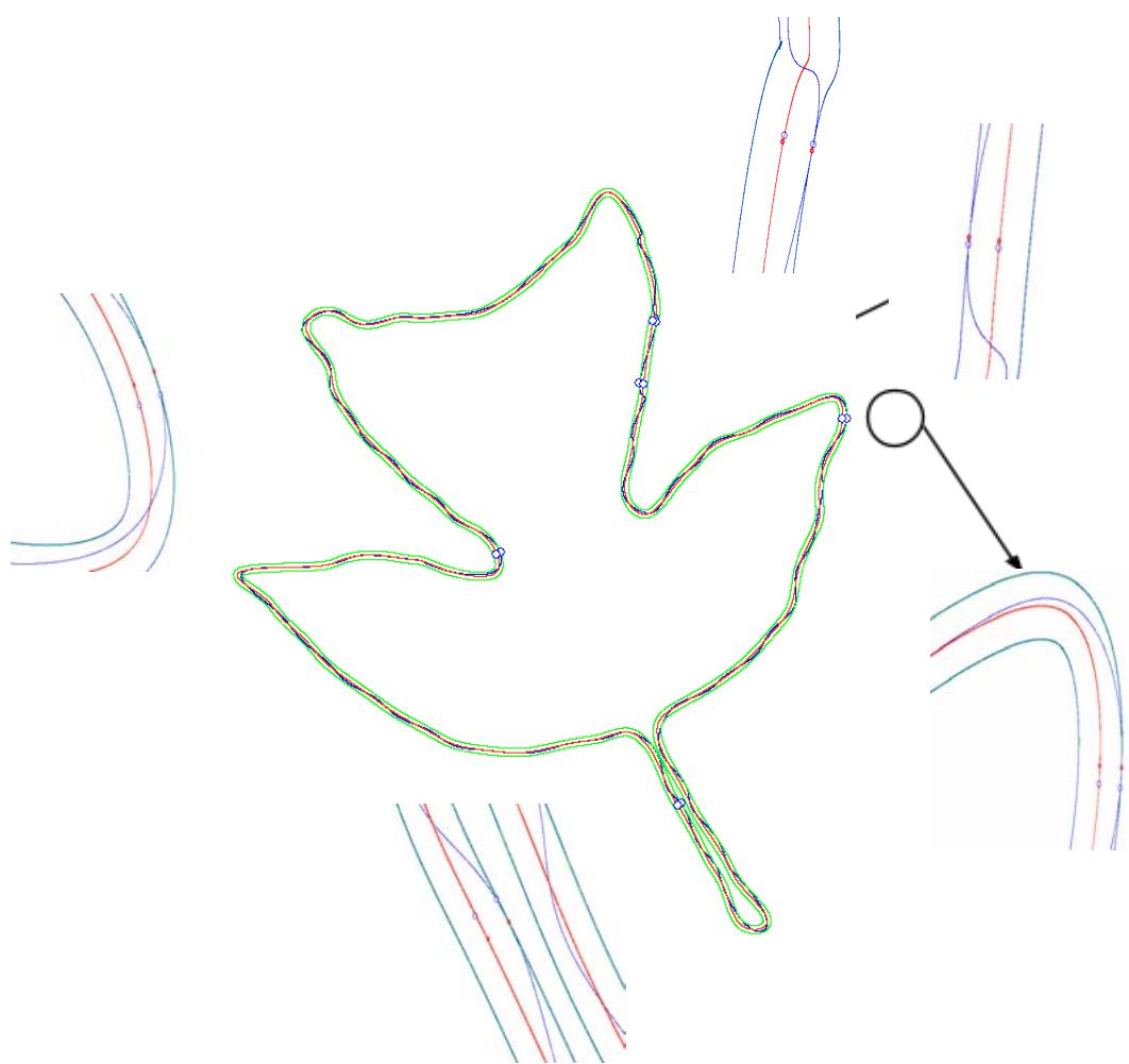 Fig. 4: Refinement of the Characteristic Points by using the Local Optimization Approaches
III. ROUNDNESS ERROR EVALUATION BASED ON THE MINIMUM ONE-SIDED HAUSDORFF DISTANCE
2.1 Introduction
In addition to being applied to the aforementioned pattern recognition and curve matching, the mathematical programming model based on the minimum one-sided Hausdorff distance can also be used in the geometric error evaluation. The relevant geometric error evaluation model is simpler and improves computational efficiency.
As the most common fits, cylindrical fits are reported to account for 80-85% of engineering applications. The measurement and evaluation of cylindrical parts are important technical approaches to ensure part precision. Currently, roundness errors are often evaluated using the minimum circumcircle, maximum incircle, least squares, and minimum area methods . Among them, the minimum area method obtains the smallest unique evaluation results, which is consistent with the roundness error definition in ANSI , ISO , and national standards . As per the minimum area evaluation method definition, two ideal concentric circles are used to contain the actual measured elements and the minimum width of the containment domain can be used to represent the roundness error. In the above evaluation process, the centre position and radius of the ideal circle can be changed. The principle for evaluating the roundness error with the minimum area method is that when the measured contour is contained by two concentric circles, at least four measured points are distributed inside and outside of two concentric circles. Since the specific algorithm used to obtain the minimum roundness error is not specified in any of the above standards , some researchers have proposed geometric error evaluation models and algorithms since the publication of these standards. In some existing studies the roundness error evaluation is regarded as a double inclusion evaluation according to the criteria of the minimum area evaluation method. In other words, there are two ideal elements that contain the actual measured elements. Based on that, the following programming algorithm can be constructed;
where, represents the coordinates of a measurement point and n represents the number of measurement points; represents the centre of an ideal circle; represents the radius of the maximum and minimum containment circles. If is arranged, R represents the radius of an ideal circle and represents the maximum and minimum normal errors. On that basis, the model from Equation (21) can be transformed into the saddle point programming model provided by a previous study ,
where, respectively represent the maximum and minimum normal errors from the point on the actual measured element to the ideal element.
The roundness error evaluation model based on the minimum one-sided Hausdorff distance is explored in the following section. Finally, the computation precision and efficiency are compared with those in Equations (21) and (22) using numerical examples.
2.2 Roundness Error Evaluation Programming Model Based on the Minimum One-Sided Hausdorff Distance
If the measured actual contour is presented as Curve A and the ideal element is presented as Curve B, the one-sided Hausdorff distance from Curve A to Curve B represents the maximum deviation from Curve A to Curve B. During the roundness error evaluation, the centre position and radius of the ideal element B can be changed and the relevant vector equation can be expressed as:
where, represents the transformation parameter vector and its components represent the circle centre coordinates and radius of the ideal element B.
From the perspective of the BUA, the one-sided Hausdorff distance between two geometric objects is the maximum deviation of the approximation object from the approximation target. The optimisation objective of the BUA is to minimise the maximum deviation under a transformation. If the approximation object scale and position parameters are selected as optimisation variables and the minimum one-sided Hausdorff distance from the approximate object to the approximation target is selected as the optimisation objective, the following roundness error evaluation programming model can be obtained after Curve A is discretised:
where, represents the shortest distance from the discrete point on Curve A to the ideal circle after transformation; represents the curve parameter corresponding to the minimum normal distance mapping mapping point of the discrete point on the ideal circle ; i represents the discrete point serial number, and m represents the total number of discrete points on Curve A. represents the similarity transformation parameter and represents the programming model optimisation variables.
It can be revealed that the optimisation model constraint function given in Equation (24) is not a linear combination of optimisation variables, but a nonlinear optimisation which needs to be linearised.
2.3 Linear Solution Method
It can be seen from the above optimisation model that the nonlinear part of the optimisation variable is included in the shortest distance . If the shortest distance in Equation (24) is regarded as a function of the transformation parameter x, it can be expressed as follows:
If the distance function is subject to Taylor's expansion at the transformation parameter zero point and their second-order and higher-order small quantities are omitted, the following expression can be obtained;
In the equation,
where, represents the shortest distance from a point on Curve A to the ideal circle B before the transformation; represents the first-order increment of the transformation parameter X, Y, R at the zero point ; represents the coordinates of the unit normal vector at a point on the ideal curve; represents the first-order partial derivative of Equation (23) for the transformation parameter X, Y, R.
After Equations (26) - (30) are substituted into Equation (24), the following linear programming model to compute the minimum one-sided Hausdorff distance between plane curves can be obtained:
where, h represents the characteristic parameter, namely the one-sided Hausdorff distance from Curve A to Curve B and m represents the number of discrete points on the actual curve.
2.4 Optimal Conditions for the Minimum Hausdorff Distance
In terms of the programming model given in Equation (24), the conditions that should be satisfied at the optimal solution point are called optimality conditions. According to the optimisation theory , the optimality condition in nonlinear programming is the K-T condition. If is the model local optimal solution, it is required to have the following K-T condition;
where, is termed a tight constraint index set and the constraint corresponding to the element in the set is termed a tight constraint.
The following expressions can be obtained from Equation (31);
After Equations (33) and (34) are substituted into the K-T condition equation (32), it can be seen that:
where, represents the vector corresponding to the tight constraint;
It is evident from previous analysis that if the characteristic point falls on the outer containment circle , it can be taken that ; If the characteristic point falls into the inner containment circle , it can be taken that . When (i = 1, 2, 3, 4), it can be found from Equation (35.c) that the 4 characteristic points cannot completely fall on the outer containment circle or the inner containment circle . This indicates that there is no characteristic point with a distribution ratio of 0:4 (4:0).
In a situation where the characteristic points' distribution ratio is 1:3 (3:1), it is safe to assume that the first characteristic point is on and the other three characteristic points are on . It can be obtained from Equations (35.a) and (35.c) that:
When Equation (36) is substituted into Equation (35.b), it can be taken that:
The geometric meaning of the above equation is that the convex combination of characteristic points 2, 3, and 4 shall contain the vector corresponding to the characteristic point 1. Since the 4 characteristic points are distinct tight constraint points, the case represented by Equation (37) cannot exist, specifically that there is no characteristic point with a distribution ratio of 1:3 (3:1).
Consequently, the characteristic points distribution ratio of the roundness error, evaluated by the minimum area method on the inner and outer containment circles and , can only be 2:2. Accordingly, the 1st and 2nd characteristic points can be arranged on and the other 2 characteristic points can be arranged on . It can be deduced from Equation (35.b) that:
Under this circumstance, it can be taken that
As suggested in Equation (39), when the roundness error evaluation results are optimal, the characteristic points on the inner and outer containment circles and are distributed as intersecting lines, which is consistent with the roundness error evaluation criteria in the minimum area method.
The K-T condition provides the necessary conditions for the optimal constrained nonlinear optimisation solution. When the optimisation objective and constraint function in the optimisation model are convex functions, the locally optimal solution is the global optimal solution. According to the optimisation theory , linear programming belongs to convex programming. Meanwhile, the linear programming model can guarantee higher precision under the assumption of small errors. Hence, the minimum condition given in Equation (35) can be regarded as a necessary and sufficient condition for reaching the global minimum.
2.5 Numerical Examples
Numerical example 1
The measured data is quoted from a previous study , as presented in Table 1. The roundness errors in the study are as follows: The centre coordinates and the radius of the ideal circle would be mm and the roundness error is 29.2816 m. Based on the data in Table 1, the conventional roundness error model (Equation 21) and the Hausdorff distance-based model (Equation 31) are compared in terms of their computation precision and efficiency.
The average value of the coordinates of 25 data points listed in Table 1 is selected as the initial circle centre coordinates . The average distance from each measurement point to the initial circle centre coordinates is selected as the initial radius of the ideal circle . A computer with a Pentium IV processor with a frequency of 2.8GHz and a 256MB memory is adopted during this process. Based on the model in Section 1.1, when the computation precision is , the centre coordinates and the radius of the ideal circle can be obtained as .
The minimum one-sided Hausdorff distance is , the roundness error is , the high characteristic points are the 11th and 18th points, and the low characteristic points are the 6th and 13th points. The average time for ten computations is 0.32ms. The results (circle centre coordinates, roundness errors, and characteristic points) from the model given in Equation (21) are similar to those computed by the model based on the minimum one-sided Hausdorff distance in Section 1.1. The radii of the maximum and minimum containment circles are 30.014702620mm and 29.985422445mm, respectively, but the average time for ten computations based on the latter is 1.73ms, which is about 5.4 times that based on the former.
Tab. 1: Initial data of Example 1
| Serial number of measure points | X-coordinate /mm | Y-coordinate/mm |
| 1 | 70.0150 | 50.0000 |
| 2 | 68.7900 | 58.4734 |
| 3 | 65.4060 | 65.9372 |
| 4 | 59.5675 | 72.7493 |
| 5 | 51.3791 | 77.7452 |
| 6 | 44.7944 | 79.6013 |
| 7 | 40.8903 | 79.9958 |
| 8 | 32.0312 | 78.9306 |
| 9 | 27.2296 | 77.1385 |
| 10 | 20.3993 | 72.7076 |
| 11 | 16.1556 | 68.2304 |
| 12 | 12.7184 | 62.4905 |
| 13 | 10.6380 | 56.0806 |
| 14 | 10.0183 | 49.2149 |
| 15 | 11.4275 | 40.8264 |
| 16 | 14.1050 | 34.8682 |
| 17 | 18.8168 | 28.7427 |
| 18 | 24.6321 | 24.2200 |
| 19 | 31.6833 | 21.1862 |
| 20 | 39.1626 | 20.0207 |
| 21 | 45.5204 | 20.5021 |
| 22 | 55.3996 | 24.2692 |
| 23 | 62.3561 | 30.0114 |
| 24 | 67.3540 | 37.6492 |
| 25 | 69.6190 | 45.2028 |
Numerical Example 2
The measured data is quoted from a previous study , as listed in Table 2. The computed results based on the steepest descent algorithm in that study are presented as follows: The ideal circle centre coordinates would be mm and the roundness error is .
The initial centre coordinates and the radius of the ideal circle are constructed via the same method as Example 1. When the computation precision is , the centre coordinates and radius of the ideal circle computed based on the minimum one-sided Hausdorff distance model would be mm, the minimum one-sided Hausdorff distance is , and the roundness error is . The 8th and 20th points are the high characteristic points and the 1st and 16th points are the low characteristic points. The average time for ten computations is 0.28ms. The results (circle centre coordinates, roundness errors, and characteristic points) computed by the model given in Equation (21) are similar to those computed by the model based on the minimum one-sided Hausdorff distance. The radii of the maximum and minimum containment circles are 30.048841860mm and 30.010610916mm, respectively, but the average time for ten computations based on the latter is 1.64ms, which is about 5.9 times that based on the former.
Tab. 2: Initial Data of Example 2
| Serial number of measure points | X-coordinate /mm | Y-coordinate /mm |
| 1 | 107.5811 | 114.2119 |
| 2 | 102.2909 | 119.9906 |
| 3 | 95.6848 | 124.2034 |
| 4 | 88.2128 | 126.5634 |
| 5 | 80.3826 | 126.9159 |
| 6 | 72.7251 | 125.2311 |
| 7 | 65.7612 | 121.6196 |
| 8 | 59.9721 | 116.3233 |
| 9 | 55.7576 | 109.7039 |
| 10 | 53.4073 | 102.2180 |
| 11 | 53.0774 | 94.3816 |
| 12 | 54.7849 | 86.7302 |
| 13 | 58.4107 | 79.7824 |
| 14 | 63.7075 | 74.0083 |
| 15 | 70.3176 | 69.8019 |
| 16 | 77.7899 | 67.4519 |
| 17 | 85.6152 | 67.1081 |
| 18 | 93.2669 | 68.7926 |
| 19 | 100.2245 | 72.4009 |
| 20 | 106.0093 | 77.6929 |
| 21 | 110.2199 | 84.3073 |
| 22 | 112.5676 | 91.7864 |
| 23 | 112.8977 | 99.6156 |
| 24 | 111.2129 | 107.2695 |
IV. CONCLUSION
-
In this study, a two-stage (rough and accurate) computation strategy was proposed to achieve the accurate computation of the minimum one-sided Hausdorff distance between continuous plane curves under a similarity transformation. A programming model for computing the minimum one-sided Hausdorff distance was developed for when the curve is provided in the form of measurement points or extremely high computation precision is not required. In addition, a programming model linearisation method was also formulated and a stable and efficient simplex method was adopted to obtain solutions. Under the conditions of continuous curves with the requirement to precisely solve the minimum one-sided Hausdorff distance, a local iterative precision algorithm, based on the programming algorithm, was established to separate the similarity transformation parameters from the curve parameters corresponding to characteristic points. Subsequently, the minimum one-sided Hausdorff distance between continuous plane curves can be accurately computed.
-
The geometrical meaning of the one-sided Hausdorff distance between plane curves and the minimum one-sided Hausdorff distance under a similarity transformation was explored. The geometrical denotation is that curve A is contained by two symmetrical equidistant curves of curve B. When the inner and outer symmetrical equidistant curves completely contain curve A with the narrowest width, half of the width value is called the one-sided Hausdorff distance from curve A to curve B. Under a similarity transformation, the geometric meaning is that when the width of the symmetric containment domain of curve B reaches the minimum, there are at least 5 tangency points between curve A and the inner and outer symmetric equidistant curves of
Curve B. The tangency points distribution ratio on the two equidistant curves can be 1:4 (4:1) or 2:3 (3:2). The maximum and minimum normal errors of curve A relative to curve B are equal in value and opposite in sign. 3. A mathematical programming model based on the minimum one-sided Hausdorff distance was applied to roundness error evaluation. Based on the local optimum condition (the K-T condition) of constrained optimisation in optimisation theory, it can be demonstrated that the minimum condition of one-sided Hausdorff distance from the actual curve to the ideal circle is equivalent to the roundness error evaluation criteria in the minimum area method specified in international and national standards. Compared with the conventional roundness error evaluation model based on the minimum area method, the optimisation objective function is the radius difference between the maximum and minimum containment circles and the number of constraint functions in the model based on the minimum one-sided Hausdorff distance is only half that in the conventional model. Therefore, the model constructed in this study can significantly improve the roundness error evaluation efficiency. Furthermore, this method can also be applied to the evaluation of other geometric errors by the minimum area method.
Declaration
Funding: This work was supported by Natural Science Foundation of Shanghai, and the Award Number is 15ZR1417200.
Conflicts of interest: We declare that we do not have any commercial or associative interest that represents a conflict of interest in connection with the work submitted.
Availability of data and material: Not applicable
Code availability: Not applicable
Authors' contributions: Improve processing efficiency and machining precision of centrifugal 3D impeller
Ethics approval: Not applicable
Consent to participate: Yes
Consent for publication: Yes
Conflict of Interest
The authors declare no conflict of interest.
Ethical Approval
Not applicable
Data Availability
The datasets used in this study are openly available at [repository link] and the source code is available on GitHub at [GitHub link].
Funding
This work did not receive any external funding.
References
Cite this article
Related Research



Special Issue
Launch a focused special issue to highlight research, emerging trends, and expert insights in your academic field.
