A Dynamic Framework for Mass-Energy Interaction: Exploring the Role of Time and Relativity

Dr. George Petropoulos

IntelliPaper

Submission received 9 May 2025
Peer Review Double Blind Handling Editor
Accepted 15 May 2025 Access Review Comments
Online published 16 June 2025

− Abstract

The relationship between mass and energy is well-established, yet the behavior of mass when interacting with energy warrants further exploration. This study examines how the introduction of time into the mass-energy interaction influences the behavior of mass. Furthermore, it investigates whether the efficient utilization of energy could potentially enable travel at speeds exceeding that of light. This paper extends the conceptualization of energy by considering mass not as a static entity but as a dynamic quantity. It explores how mass distributes received energy and its behavior under various values of energy and time. The investigation begins with the fundamental form of mass, specifically the point energy mass, which is influenced by both energy and time. The study then expands to encompass larger and more complex forms of mass, analyzing the generalized effects of energy and time on their behavior. Additionally, the study examines the roles of space and speed in relation to energy and time, incorporating in the investigation fundamental equations of relativity. The findings suggest the possibility of mass traveling at speeds that would be considered as limited until now, by setting appropriate mass factors.

− Explore Digital Article Text

I. INTRODUCTION

This study investigates energy distribution equations and models within mass structures and the behavioral transformations exhibited by mass following energy absorption, which explain the relation of mass with energy and time which is missing from current framework. The research extends beyond prior studies by employing a dynamic approach to analyze mass, tracking its temporal evolution from initial energy configurations to bigger and complex forms of mass. However, previous models are used to investigate relation with the limitations that these models apply, such as the speed limit a mass can travel.

The methodological framework commences with an examination of how point energy mass responds to energy while evolving over time. Traditional energy expressions reveal limitations when mass is held constant, with spatial changes considered solely as time-dependent functions. This framework challenges these traditional conceptualizations by exploring energy distribution to mass, thereby enabling a comprehensive study of resultant mass behaviors.

This expanded perspective on energy distribution results in differential equations that incorporate energy, time, space, and mass. Solutions to these equations uncover fundamental connections between space and speed and energy and time offering insights into potential mass transit at speeds, possibly, higher than light, initially being considered at theoretical level. Two- and three-dimensional visualizations depict individual variable changes against energy and time durations, illustrating their combined effects.

II. METHODOLOGY

There are two ways to approach the relation between energy and mass. The one is the classical that combines various expressions of energy, including potential energy and kinetic energy, whereas the second approach is the relativistic one.

Starting the investigation with the classical expression, let us consider a mass that is located at a height h from the surface of earth. The potential energy at this height is calculated as:

E_{p} = m \cdot g \cdot h

where g is the gravitational field strength and h is the measure of height h.

If the mass is let it moves towards the ground and the potential energy is transformed to kinetic energy. Just before touching the ground the kinetic energy of the mass is calculated as:

E_{k} = \frac{1}{2} m \cdot |\vec{u}|^{2}

Where is the magnitude of the speed of mass just before touching the ground and is calculated as:

| \vec {u} | = \sqrt {2 \cdot g \cdot h}\tag{3}

At any position n the energy of mass is:

\mathrm{E}_{n} = \frac{1}{2} \mathrm{m} \cdot |\vec{u}_{n}|^{2} + \mathrm{m} \cdot \mathrm{g} \cdot \mathrm{h}_{n}

As it is widely known, if the gravitational field strength g is dimensionally analysed, it is measured in units (5). If the term (6) is considered as second derivative, then the gravity constant would imply the second derivative of mass. This makes one wonder if there could be another way to express mass so that the term has a logical meaning.

The energy of a mass is measured in Joule (J), the dimensional analysis of which is: . In this case it can be considered that the energy a mass holds is expressed by the contribution of the space squared, the mass, and the reverse time squared. The existence of reverse time can be considered a differentiation of a quantity over time.

2.1. analysis of the model

In general, when studying energy, it is considered that the differentiation over time applies only to space. However, it has been proven that mass is also time-dependent, and the generic expression of point energy mass (pem) in such a case is:

\mathrm{m} \left(\varepsilon , \vec{s}, t\right) = \mu_{0,\mathrm{g}} \mathrm{e}^{\mathrm{i}\left(\theta\left(t\right) + \theta\left(\varepsilon\right) - \theta\left(\vec{s}\right) + \varphi\right)}

so that:

\mu_{0,\mathrm{g}} = \mathbf{g}_{\varepsilon} \mathbf{g}_{\mathrm{t}} \mathbf{g}_{\vec{s}}^{’}\tag{9}

and

\mathbf{g}_{\mathrm{t}} = \sqrt{\frac{1}{\omega^{4}} + (C_{1}^{'\,}\mathbf{t} + C_{2}^{'})^{2} - \frac{2}{\omega^{2}} (C_{1}^{'\,}\mathbf{t} + C_{2}^{'}) \cos(\omega (\mathbf{t} - \mathbf{t}_{1}))}, |\mathbf{g}(\mathbf{t})| \geq 0

\mathrm{g}_{\varepsilon} = \frac{2}{\alpha} \sin \left(\frac{\alpha}{2} (\varepsilon - \varepsilon_{1})\right)\tag{11}

and\theta(\varepsilon) = \frac{\alpha}{2}(\varepsilon + \varepsilon_{1})

\mathbf{g}_{\vec{s}}' = |\mathbf{g}'(\vec{s})| = \frac{1}{\sqrt{c_{k}^{2} + (\lambda\vec{k}\cdot\vec{s} + \lambda_{v})^{2} - 2c_{k}\lambda(\vec{k}\cdot\vec{s} + c_{\lambda})\cos(\vec{k}\cdot(\vec{s} - \vec{s}_{0}))}}

\tan\theta(t) = \frac{\sin(\omega t) - \omega^{2}(C_{1}^{' }t + C_{2}^{'})\sin(\omega t_{1})}{\cos(\omega t) - \omega^{2}(C_{1}^{' }t + C_{2}^{'})\cos(\omega t_{1})}

Also:

\theta (\varepsilon) = \frac{\alpha}{2} (\varepsilon + \varepsilon _ {1})

\tan\theta(\vec{s}) = \frac{-c_{\kappa}\sin(\vec{k}\cdot\vec{s}) + \lambda(\vec{k}\cdot\vec{s}+c_{\lambda})\sin(\vec{k}\cdot\vec{s}_{0})}{-c_{\kappa}\cos(\vec{k}\cdot\vec{s}) + \lambda(\vec{k}\cdot\vec{s}+c_{\lambda})\cos(\vec{k}\cdot\vec{s}_{0})}

Another expression of mass that derives from the analysis of the factor is:

m(\varepsilon, \vec{s}, t) = |\mu_{\mathrm{A}}| e^{i\varphi_{\mu\mathrm{A}}} - |\mu_{\mathrm{B}}| e^{i\varphi_{\mu\mathrm{B}}}

considering:

|\mu_{A}(\varepsilon)| = \mu_{0,\varepsilon} = 2 \frac{|\vec{\kappa}|^{2}}{\alpha \omega^{2}} \sin\left(\frac{\alpha}{2}(\varepsilon - \varepsilon_{1})\right) \geq 0

and

\varphi_ {\mu_ {A}} = \omega t - \vec{k} \cdot \vec{s} - \frac{\alpha}{2} (\varepsilon_ {1} + \varepsilon) + \varphi\tag{19}

Also:

|\mu_ {B} (\varepsilon) | = 2 \frac{| \vec{\kappa} | ^ {2}}{\alpha \omega^ {2}} \sin \left(\frac{\alpha}{2} (\varepsilon - \varepsilon_ {1})\right) \omega^ {2} (C _ {1} ^ {\prime} t + C _ {2} ^ {\prime}) \geq 0

and

\varphi_ {\mu_ {B}} = \omega t _ {1} - \vec{k} \cdot \vec{s} - \frac{\alpha}{2} (\varepsilon_ {1} + \varepsilon) + \varphi

In other words:

m(\varepsilon, \vec{s}, t) = \mu_{0,\varepsilon} e^{i(\omega t - \vec{k}\cdot\vec{s} + \frac{\alpha}{2}(\varepsilon_1 + \varepsilon) + \varphi)} - \mu_{0,\varepsilon} \omega^2 (C_1' t + C_2') e^{i(\omega t_1 - \vec{k}\cdot\vec{s} + \frac{\alpha}{2}(\varepsilon_1 + \varepsilon) + \varphi)}

If the quantities of space and energy contained are considered constants, the mass can be expressed as time-dependent as follows:

m (t) = \mu_ {0} \mathrm{e} ^ {\mathrm{i} (\omega t + \theta)} - \omega^ {2} \mu_ {0} (C _ {1} ^ {\prime} t + C _ {2} ^ {\prime}) \mathrm{e} ^ {\mathrm{i} (\omega t _ {1} + \theta)}\tag{23}

whereas the generic format, as expressed in equation (1), considering only the time as the variable, is:

\mathbf{m}(t) = \mu_{0,g} \mathrm{e}^{\mathrm{i} (\theta(t) + \varphi)}

Considering the dimensional analysis of Joule (J), the competition of time is expressed as (25), which can also be expressed as (26). If this approach is combined with the expression of mass developed in relations (8) and (23), the differentiation over time can apply not only to the quantity of space but also to the quantity of mass. Then, starting through the dimensional analysis, the Joule expression can be expressed as follows:

J = \frac {(k g)}{(s ^ {2})} \cdot (m ^ {2}) + \frac {(k g)}{(s)} \cdot \frac {(m ^ {2})}{(s)} + (k g) \cdot \frac {(m ^ {2})}{(s ^ {2})}\tag{27}

which, in terms of the respective quantities, is expressed on one axis as:

E = \frac {d ^ {2} m}{d t ^ {2}} \cdot x ^ {2} + \frac {d m}{d t} \cdot \frac {d x ^ {2}}{d t} + m \cdot \frac {d ^ {2} x ^ {2}}{d t ^ {2}}\tag{28}

or, in a simpler expression:

E = \ddot{m} \cdot x^{2} + \dot{m} \cdot \dot{x}^{2} + m \cdot \ddot{x}^{2}

Going further and implementing the differentiation on the core term, i.e., [6],[7],[8], [9], the result is:

(30)

\frac{d^{2}}{dt^{2}}(m\cdot\vec{x}^{2}) = \frac{d^{2}m}{dt^{2}}\cdot\vec{x}^{2} + 4\cdot\frac{dm}{dt}\cdot\vec{x}\cdot\frac{dx}{dt} + 2\cdot m\cdot\vec{x}\cdot\frac{d^{2}\vec{x}}{dt^{2}} + 2\cdot m\cdot\left(\frac{d\vec{x}}{dt}\right)^{2}

Then, the energy provided to the mass is expressed as [6],[7],[8],:

E = \frac {d ^ {2} m}{d t ^ {2}} \cdot \vec {x} ^ {2} + 4 \cdot \frac {d m}{d t} \cdot \vec {x} \cdot \frac {d x}{d t} + 2 \cdot m \cdot \vec {x} \cdot \frac {d ^ {2} \vec {x}}{d t ^ {2}} + 2 \cdot m \cdot \left(\frac {d \vec {x}}{d t}\right) ^ {2}\tag{32}

which, in a simpler format, is expressed as [6],[7],[8], :

E = \ddot{m} \vec{x}^2 + 4 \dot{m} \vec{x} \cdot (\dot{\vec{x}}) + 2 m \vec{x} \cdot (\ddot{\vec{x}}) + 2 m (\dot{\vec{x}})^2

The derivatives of mass based on relation (23) are [10],[11], [12],:

\frac {\mathrm{d} m}{\mathrm{d} t} = \frac {\mathrm{d}}{\mathrm{d} t} \big (\mu_ {0} e ^ {i (\omega t + \theta)} - \omega^ {2} \mu_ {0} (C _ {1} ^ {\prime} t + C _ {2} ^ {\prime}) e ^ {i (\omega t _ {1} + \theta)} \big)\tag{34}

or

\frac{\mathrm{d} \mathbf{m}}{\mathrm{d} t} = \dot{\mathbf{m}} = \mathrm{i} \omega \mu_0 \mathrm{e}^{\mathrm{i} (\omega t + \theta)} - \omega^2 \mu_0 C_1' \mathrm{e}^{\mathrm{i} (\omega t_1 + \theta)}

The second derivative is calculated as:

\frac {\mathrm{d} \mathsf {m}}{\mathrm{d} t ^ {2}} = \frac {\mathrm{d}}{\mathrm{d} t} \big (\mathrm{i} \omega \mu_ {0} \mathrm{e} ^ {\mathrm{i} (\omega t + \theta)} - \omega^ {2} \mu_ {0} C _ {1} ^ {\prime} \mathrm{e} ^ {\mathrm{i} (\omega t _ {1} + \theta)} \big)\tag{36}

or

\frac{\mathrm{dm}}{\mathrm{dt}^{2}} = \ddot{\mathrm{m}} = -\omega^{2}\mu_{0}\mathrm{e}^{\mathrm{i}(\omega t + \theta)}

The implementation of the mass differentiation, basis relations (34) up to (37) on equation (33) provides:

\begin{array}{c} E = (- \omega^ {2} \mu_ {0} e ^ {i (\omega t + \theta)}) \vec {x} ^ {2} + 4 (i \omega \mu_ {0} e ^ {i (\omega t + \theta)} - \omega^ {2} \mu_ {0, \varepsilon} C _ {1} ^ {\prime} e ^ {i (\omega t _ {1} + \theta)}) \vec {x} \cdot (\dot {\vec {x}}) + 2 \mu_ {0} (e ^ {i (\omega t + \theta)} - \\\omega^ {2} (C _ {1} ^ {\prime} t + C _ {2} ^ {\prime}) e ^ {i (\omega t _ {1} + \theta)}) ((\vec {x} \cdot (\ddot {\vec {x}}) + (\dot {\vec {x}}) ^ {2}) \end{array}\tag{38}

Since mass is composed of two terms, and , it can be considered that the energy can be distributed to these two terms and can be split to and so that each energy term can be assigned to each mass term. Then it is:

\mathrm {E_ {A}} = - \omega^ {2} \mu_ {0} \mathrm{e} ^ {\mathrm{i} (\omega t + \theta)} \vec {\mathrm{x}} ^ {2} + 4 \mathrm{i} \omega \mu_ {0} \mathrm{e} ^ {\mathrm{i} (\omega t + \theta)} \vec {\mathrm{x}} \cdot (\dot {\vec {\mathrm{x}}}) + 2 \mu_ {0} \mathrm{e} ^ {\mathrm{i} (\omega t + \theta)} ((\vec {\mathrm{x}} \cdot (\ddot {\vec {x}}) + (\dot {\vec {\mathrm{x}}}) ^ {2})\tag{39}

and

\mathrm{E} _ {\mathrm{B}} = - 4 \omega^ {2} \mu_ {0} C _ {1} ^ {\prime} \mathrm{e} ^ {\mathrm{i} (\omega t _ {1} + \theta)}) \vec {\mathrm{x}} \cdot (\dot {\vec {\mathrm{x}}}) - 2 \omega^ {2} \mu_ {0} (C _ {1} ^ {\prime} t + C _ {2} ^ {\prime}) \mathrm{e} ^ {\mathrm{i} (\omega t _ {1} + \theta)}) ((\vec {\mathrm{x}} \cdot (\ddot {\vec {\mathrm{x}}}) + (\dot {\vec {\mathrm{x}}}) ^ {2})\tag{40}

In the case that two or more masses are added for the creation of a bigger one, the new mass is:

m _ {T} = m _ {0 T} e ^ {i \varphi_ {T}}\tag{41}

so that:

m _ {0 T} = | m _ {T} | = \sqrt {\sum_ {i = 1} ^ {n} \mu_ {0 , i} ^ {2} + 2 \sum_ {i = 1} ^ {n - 1} \sum_ {j = i + 1} ^ {n} \mu_ {0 , i} \mu_ {0 , j} c o s (\theta_ {i} - \theta_ {i})}\tag{42}

and

tan\varphi_T = \frac{\sum_{i=1}^{n} sin(\omega_i t) - \sum_{i=1}^{n} \omega_i^2 (C'_1,t + C'_2,i) sin(\omega_i t_1,i)}{\sum_{i=1}^{n} cos(\omega_i t) - \sum_{i=1}^{n} \omega_i^2 (C'_1,t + C'_2,i) cos(\omega_i t_1,i)}

In which is the total number of masses that contribute to creating the bigger mass and and .

In such a case, equation (26) becomes:

E = \ddot {m} _ {T} \vec {x} ^ {2} + 4 \dot {m} _ {T} \vec {x} \cdot (\dot {\vec {x}}) + 2 m _ {T} ((\vec {x} \cdot (\ddot {\vec {x}}) + (\dot {\vec {x}}) ^ {2})\tag{44}

Equation (45) is an expanded expression of the energy of a mass at a random position and includes all possible forms of energy of the mass at that position, e.g. kinetic energy, potential energy and forms of energy that are associated with the time-dependent format of mass.

In the case that the mass is considered as a solid object it is:

\dot{m}_{T} = \ddot{m}_{T} = 0

Then equation (44) turns into:

E = 2 m _ {T} \vec {x} \cdot (\ddot {\vec {x}}) + 2 m _ {T} (\dot {\vec {x}}) ^ {2}\tag{46}

which of the same format as equation (4).

2.2 Relativistic Approach

The relativity has been developed in order to expand and complete the Newtonia mechanics as there were a number of issues that could be explained by them , , . In order to make the investigation complete in context, since this paper refers to the quantities of energy, mass, space and time, it is of paramount importance. to include relativistic equations, taking the total energy of a mass as [17], [18], :

\mathrm{E} = \gamma \mathrm{m} _ {0} c ^ {2}\tag{47}

so that:

\gamma = \frac{1}{\sqrt{1 - \frac{u^{2}}{c^{2}}}}\tag{48}

where u is the speed of the mass and c is the speed of light.

In this case both the simple format of cem as well the generic format are investigated.

Considering that (47) expresses the total energy of the mass, it can be combined with (39), (40) and (44) and provide the modified equations. In this respect equation (39) is:

E _ {A} = - \omega^ {2} \mu_ {0} e ^ {i (\omega t + \theta)} \vec {x} ^ {2} + 4 i \omega \mu_ {0} e ^ {i (\omega t + \theta)} \vec {x} \cdot (\dot {\vec {x}}) + 2 \mu_ {0} e ^ {i (\omega t + \theta)} ((\vec {x} \cdot (\ddot {\vec {x}}) + (\dot {\vec {x}}) ^ {2})\tag{49}

or

\mathrm{k} _ {\mathrm{A}} \gamma \mathrm{m} _ {0} c ^ {2} = - \omega^ {2} \mu_ {0} \mathrm{e} ^ {\mathrm{i} (\omega t + \theta)} \vec {\mathrm{x}} ^ {2} + 4 \mathrm{i} \omega \mu_ {0} \mathrm{e} ^ {\mathrm{i} (\omega t + \theta)} \vec {\mathrm{x}} \cdot (\dot {\vec {\mathrm{x}}}) + 2 \mu_ {0} \mathrm{e} ^ {\mathrm{i} (\omega t + \theta)} ((\vec {\mathrm{x}} \cdot (\ddot {\vec {x}}) + (\dot {\vec {\mathrm{x}}}) ^ {2})\tag{50}

Whereas equation (33) becomes:

\mathrm{E} _ {\mathrm{B}} = - 4 \omega^ {2} \mu_ {0} C _ {1} ^ {\prime} \mathrm{e} ^ {\mathrm{i} (\omega t _ {1} + \theta)}) \vec {\mathrm{x}} \cdot (\dot {\vec {\mathrm{x}}}) - 2 \omega^ {2} \mu_ {0} (C _ {1} ^ {\prime} t + C _ {2} ^ {\prime}) \mathrm{e} ^ {\mathrm{i} (\omega t _ {1} + \theta)}) ((\vec {\mathrm{x}} \cdot (\ddot {\vec {\mathrm{x}}}) + (\dot {\vec {\mathrm{x}}}) ^ {2})\tag{51}

or

\mathrm {k_ {B} \gamma m_ {0} c^ {2} = - 4 \omega^ {2} \mu_ {0} C_ {1} ^ {\prime} e^ {i(\omega t_ {1} + \theta)}) \vec {x} \cdot (\dot {\vec {x}}) - 2 \omega^ {2} \mu_ {0} (C_ {1} ^ {\prime} t+ C_ {2} ^ {\prime}) e^ {i(\omega t_ {1} + \theta)}) ((\vec {x} \cdot (\ddot {\vec {x}}) + (\dot {\vec {x}}) ^ {2})}\tag{52}

Finally, equation (45) becomes:

E = \ddot {m} _ {T} \vec {x} ^ {2} + 4 \dot {m} _ {T} \vec {x} \cdot (\dot {\vec {x}}) + 2 m _ {T} ((\vec {x} \cdot (\ddot {\vec {x}}) + (\dot {\vec {x}}) ^ {2})\tag{53}

or

\gamma m_{0} c^{2} = \ddot{m}_{T} \vec{x}^{2} + 4 \dot{m}_{T} \vec{x} \cdot (\dot{\vec{x}}) + 2 m_{T} (\vec{x} \cdot \ddot{\vec{x}} + \dot{\vec{x}}^{2})

considering the total energy of the mass is calculated as per the relativistic approach.

\text { III. RESULTS }

When the solutions of equations (39) and (40), derived from the mathematical process, are applied for a single axis (so that i=1 or 2 or 3 in the case of a 3-dimensional Euclidean space), the general results remain unaltered.

The solution of equation (39) provides:

A. Space:

The solution of the differential equation of the real part provides:

\mathrm{x}_{i,Re}(\mathrm{t}) = \pm \frac{\sqrt{-\frac{\mathrm{E}_{\mathrm{A}}}{\mu_{0}} \cos(\omega t + \theta) + \mathrm{k}_{1} \omega \mathrm{e}^{\omega t} + \mathrm{k}_{2} \omega^{2} \mathrm{e}^{-\omega t}}}{\sqrt{2} \omega}

where:

- \frac{\mathrm{E_ {A}}}{\mu_ {0}} \cos (\omega t + \theta) + \mathrm{k_ {1} \omega e^ {\omega t}} + \mathrm{k_ {2} \omega^ {2} e^ {- \omega t}} \geq 0

and

\omega \neq 0\tag{57}

The solution of the differential equation of the imaginary part provides:

x_{i,Im}(t) = \pm \frac{\sqrt{\frac{\mathrm{E}_{\mathrm{A}}}{\mu_0} \cos(\omega t + \theta) + k_3 \omega^2}}{\sqrt{2} \omega}\tag{58}

where:

\frac {\mathrm{E} _ {\mathrm{A}}}{\mu_ {0}} \cos (\omega t + \theta) + \mathrm{k} _ {3} \omega^ {2} \geq 0\tag{59}

and

\omega \neq 0

B. Speed:

The differentiation of the relations (55) and (58) yields the speed, which, for equation (55), is calculated as:

\dot{x}_{i,Re}(t) = \pm \frac{e^{-\omega t} (\frac{E_{A}}{\mu_0} \sin(\omega t + \theta) e^{\omega t} + \omega (k_1 e^{2\omega t} - k_2 \omega))}{2\sqrt{2} \sqrt{- \frac{E_{A}}{\mu_0} \cos(\omega t + \theta) + k_1 \omega e^{\omega t} + k_2 \omega^2 e^{-\omega t}}}

with the restriction:

- \frac{\mathrm{E}_{\mathrm{A}}}{\mu_{0}} \cos(\omega t + \theta) + k_{1} \omega e^{\omega t} + k_{2} \omega^{2} e^{-\omega t} > 0

whereas the differentiation of equation (58) provides:

\dot{x}_{i,Im}(t) = \mp \frac{\frac{\mathrm{E}_\mathrm{A}}{\mu_0} \sin(\omega t + \theta)}{\sqrt{\frac{\mathrm{E}_\mathrm{A}}{\mu_0} \cos(\omega t + \theta) + k_3 \omega^2}}

where the restriction that applies is:

\frac{\mathrm{E_ {A}}}{\mu_ {0}} \cos (\omega t + \theta) + k_3 \omega^2 > 0

Additionally, the equations that are derived from (58) are:

A. Space:

\begin{array}{c} \mathrm{x} _ {i, R e} (\mathrm{t}) \\= \pm \frac {\sqrt {- \frac {\mathrm{E} _ {\mathrm{B}}}{2 \omega^ {2} \mu_ {0}} c o s (\omega t _ {1} + \theta) \left(C _ {1} ^ {\prime 2} t ^ {2} + C _ {1} ^ {\prime} C _ {2} ^ {\prime} t + C _ {2} ^ {\prime 2}\right) + k _ {4} C _ {1} ^ {\prime} + 2 k _ {5} C _ {1} ^ {\prime 2} (C _ {2} ^ {\prime} t + C _ {2} ^ {\prime})}}{C _ {1} ^ {\prime} \sqrt {(C _ {1} ^ {\prime} t + C _ {2} ^ {\prime})}} \end{array}\tag{64}

The restrictions that apply are:

- \frac {\mathrm {E_ {B}}}{2 \omega^ {2} \mu_ {0}} c o s (\omega t _ {1} + \theta) \big (C _ {1} ^ {' 2} t ^ {2} + C _ {1} ^ {'} C _ {2} ^ {'} t + C _ {2} ^ {' 2} \big) + k _ {4} C _ {1} ^ {'} + 2 k _ {5} C _ {1} ^ {' 2} (C _ {2} ^ {'} t + C _ {2} ^ {'}) \geq 0\tag{65}

and

C _ {1} ^ {\prime} t + C _ {2} ^ {\prime} > 0 a n d C _ {1} ^ {\prime} \neq 0\tag{66}

B. Speed:

\dot {\mathbf {x}} _ {i, R e} (t)

= \mp \frac {C _ {1} ^ {\prime} \left(\frac {\mathrm{E} _ {\mathrm{B}}}{2 \omega^ {2} \mu_ {0}} c o s (\omega t _ {1} + \theta) t (C _ {1} ^ {\prime} t + C _ {2} ^ {\prime})\right) + k _ {4}}{2 (C _ {1} ^ {\prime} t + C _ {2} ^ {\prime})) ^ {\frac {3}{2}} \sqrt {- \frac {\mathrm{E} _ {\mathrm{B}}}{2 \omega^ {2} \mu_ {0}} c o s (\omega t _ {1} + \theta) \big (C _ {1} ^ {\prime 2} t ^ {2} + C _ {1} ^ {\prime} C _ {2} ^ {\prime} t + C _ {2} ^ {\prime 2} \big) + C _ {1} ^ {\prime} (2 k _ {5} C _ {1} ^ {\prime} (C _ {1} ^ {\prime} t + C _ {2} ^ {\prime}) + k _ {4})}}\tag{67}

where the restrictions for this case are:

- \frac {\mathrm {E_ {B}}}{2 \omega^ {2} \mu_ {0}} c o s (\omega t _ {1} + \theta) \big (C _ {1} ^ {\prime 2} t ^ {2} + C _ {1} ^ {\prime} C _ {2} ^ {\prime} t + C _ {2} ^ {\prime 2} \big) + C _ {1} ^ {\prime} (2 k _ {5} C _ {1} ^ {\prime} (C _ {1} ^ {\prime} t + C _ {2} ^ {\prime}) + k _ {4}) > 0

C _ {1} ^ {\prime} t + C _ {2} ^ {\prime} > 0

Equation (40) provides solutions only from the real part, while the solutions derived from the imaginary part of equation (40) define a point or set of points where this relation applies. These can be expressed as follows:

in case , then ,

(69) 2. in case , then , , which is not the case since it is desired that

(70) To combine equations with (56) and (51) with (59), it is considered that:

E = \mathrm {E_ {A}} + \mathrm {E_ {B}}\tag{71}

It can be set:

\mathrm{E} _ {\mathrm{A}} = k _ {E} E\tag{72}

and

\mathrm{E} _ {\mathrm{B}} = (1 - k _ {E}) E\tag{73}

so that the factor :

k _ {E} \in [ 0, 1 ] \subset \mathbb {R}\tag{74}

expresses how energy is distributed between the two parts of mass.

In addition, the quantity E expresses the total energy supplied to the mass.

The combination of equations (71) up to (74) with (55), (58), (52), (54), (56) and (59) provide the following results:

Space: The solution of the real part provides two terms, each affecting the change of space depending on the time and energy supplied to the mass. In this respect, the equation that expresses the space is the sum of both terms on each axis. Taking into consideration the equations (54) and (66) in combination with (62) and (63), the expressions of space are derived as follows:

For the real part:

\begin{array}{r l} & {\mathrm{x} _ {i, R e} (\mathrm{E}, t)} \\& {= \pm \frac {\sqrt {- \frac {k _ {E} E}{\mu_ {0}} \cos (\omega t + \theta) + k _ {1} \omega e ^ {\omega t} + k _ {2} \omega^ {2} e ^ {- \omega t}}}{\sqrt {2} \omega}} \\& {\pm \frac {\sqrt {- \frac {(1 - k _ {E}) E}{2 \omega^ {2} \mu_ {0}} c o s (\omega t _ {1} + \theta) (C _ {1} ^ {\prime 2} t ^ {2} + C _ {1} ^ {\prime} C _ {2} ^ {\prime} t + C _ {2} ^ {\prime 2}) + k _ {4} C _ {1} ^ {\prime} + 2 k _ {5} C _ {1} ^ {\prime 2} (C _ {2} ^ {\prime} t + C _ {2} ^ {\prime})}}{\sqrt {C _ {1} ^ {\prime 2} (C _ {1} ^ {\prime} t + C _ {2} ^ {\prime})}}} \end{array}\tag{75}

For the imaginary part:

x _ {i, I m} (E, t) = \pm \frac {\sqrt {\frac {k _ {E} E}{\mu_ {0}} \cos (\omega t + \theta) + k _ {3} \omega^ {2}}}{\sqrt {2} \omega}\tag{76}

Speed: The solution of the real part provides two terms, each depending on time and energy. In this respect, the equations that express speed are the sum of both terms on each axis. Taking into consideration the equations (63) and (66), in combination with (61) and (72), the expressions of speed yielded as follows:

Real part:

\begin{array}{r l} & {\dot {x} _ {i, R e} (t)} \\& = \pm \frac {\frac {k _ {E} E}{\mu_ {0}} \sin (\omega t + \theta) + k _ {1} \omega e ^ {\omega t} - k _ {2} \omega^ {2} e ^ {- \omega t}}{2 \sqrt {2} \sqrt {- \frac {k _ {E} E}{\mu_ {0}} \cos (\omega t + \theta) + k _ {1} \omega e ^ {\omega t} + k _ {2} \omega^ {2} e ^ {- \omega t}}} \\& {\mp \frac {C _ {1} ^ {\prime} \left(\frac {(1 - k _ {E}) E}{2 \omega^ {2} \mu_ {0}} c o s (\omega t _ {1} + \theta) t (C _ {1} ^ {\prime} t + 2 C _ {2} ^ {\prime}) + k _ {4}\right)}{2 (C _ {1} ^ {\prime} t + C _ {2} ^ {\prime})) ^ {\frac {3}{2}} \sqrt {- \frac {(1 - k _ {E}) E}{2 \omega^ {2} \mu_ {0}} c o s (\omega t _ {1} + \theta) \bigl (C _ {1} ^ {\prime 2} t ^ {2} + C _ {1} ^ {\prime} C _ {2} ^ {\prime} t + C _ {2} ^ {\prime 2} \bigr) + C _ {1} ^ {\prime} (2 k _ {5} C _ {1} ^ {\prime} (C _ {1} ^ {\prime} t + C _ {2} ^ {\prime}) + k _ {4})}}} \end{array}\tag{77}

Imaginary part:

\dot {x} _ {i, I m} (t) = \mp \frac {\frac {k _ {E} E}{\mu_ {0}} \sin (\omega t + \theta)}{2 \sqrt {\frac {k _ {E} E}{\mu_ {0}} \cos (\omega t + \theta) + k _ {3} \omega^ {2}}}\tag{78}

The mathematical process for the solution of equation (44) is more complicated, and various solutions have been proposed. One of the solutions proposed considers .

Again, for the solution of this equation, it is assumed that the use of a single axis does not affect the generality of the results; in this case, the study focuses on the axis . The equations that express space are:

Real part:

\mathrm{x} _ {i, R e} (\mathrm{t}) = \pm \frac {\sqrt {- \frac {E}{m _ {0 T}} \cos (p _ {1} t + p _ {2}) + p _ {3} p _ {1} \mathrm{e} ^ {p _ {1} \mathrm{t}} + p _ {4} p _ {1} ^ {2} \mathrm{e} ^ {- p _ {1} \mathrm{t}}}}{\sqrt {2} p _ {1}}\tag{79}

where the applicable restrictions are:

- \frac {E}{m _ {0 T}} \cos (p _ {1} t + p _ {2}) + p _ {3} p _ {1} \mathrm{e} ^ {p _ {1} \mathrm{t}} + p _ {4} p _ {1} ^ {2} \mathrm{e} ^ {- p _ {1} \mathrm{t}} \geq 0\tag{80}

p _ {1} \neq 0\tag{81}

Imaginary part:

x _ {i, I m} (t) = \pm \frac {\sqrt {\frac {E}{m _ {0 T}} \cos (p _ {1} t + p _ {2}) + p _ {5} p _ {1} ^ {2}}}{\sqrt {2} p _ {1}}\tag{82}

where the restrictions are:

\frac {E}{m _ {0 T}} c o s (p _ {1} t + p _ {2}) + p _ {5} p _ {1} ^ {2} \geq 0\tag{83}

and

p _ {1} \neq 0

The equations of speed that are produced from the equation (82) is:

\dot {x} _ {i, I m} (t) = \mp \frac {\frac {E}{m _ {0 T}} \sin (p _ {1} t + p _ {2})}{2 \sqrt {\frac {E}{m _ {0 T}} \cos (p _ {1} t + p _ {2}) + p _ {5} p _ {1} ^ {2}}}\tag{84}

having as restriction:

\frac {E}{m _ {0 T}} c o s (p _ {1} t + p _ {2}) + p _ {5} p _ {1} ^ {2} > 0\tag{85}

Whereas the speed that is produced from equation (79) is:

\dot {x} _ {i, R e} (t) = \pm \frac {\frac {E}{m _ {0 T}} \sin (p _ {1} t + p _ {2}) + p _ {3} p _ {1} \mathrm{e} ^ {p _ {1} t} - p _ {4} p _ {1} ^ {2} \mathrm{e} ^ {- p _ {1} t}}{2 \sqrt {2} \sqrt {- \frac {E}{m _ {0 T}} \cos (p _ {1} t + p _ {2}) + p _ {3} p _ {1} \mathrm{e} ^ {p _ {1} t} + p _ {4} p _ {1} ^ {2} \mathrm{e} ^ {- p _ {1} t}}}\tag{86}

The applicable restriction is:

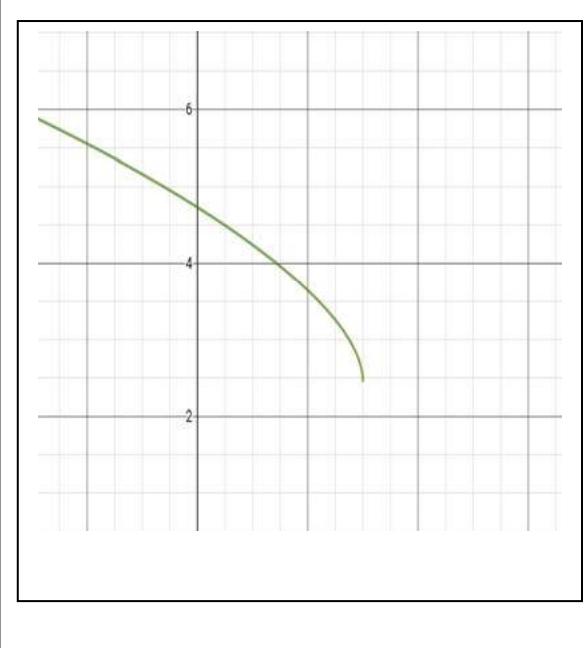
- \frac {E}{m _ {0 T}} \cos (p _ {1} t + p _ {2}) + p _ {3} p _ {1} \mathrm{e} ^ {p _ {1} \mathrm{t}} + p _ {4} p _ {1} ^ {2} \mathrm{e} ^ {- p _ {1} \mathrm{t}} > 0\tag{87}

The equations (75), (76), (77), (78), as well as (79), (82), (84) and (86), are represented by the figures below, using energy and time as parameters.

Figure 1: Graphical representation of real part of space dependent on energy based on equation (75)

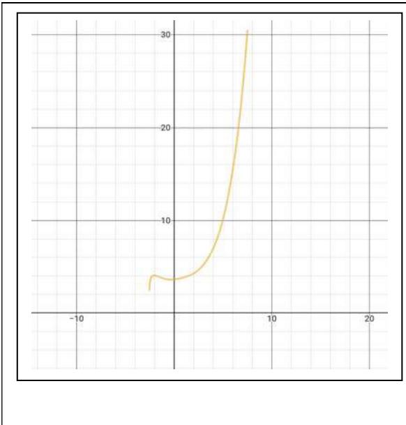Figure 3: Graphical representation of real part of space dependent on time, based on equation (75)

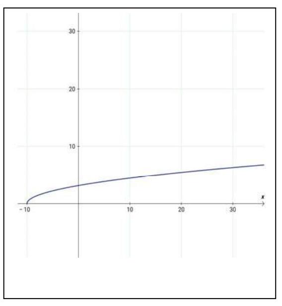
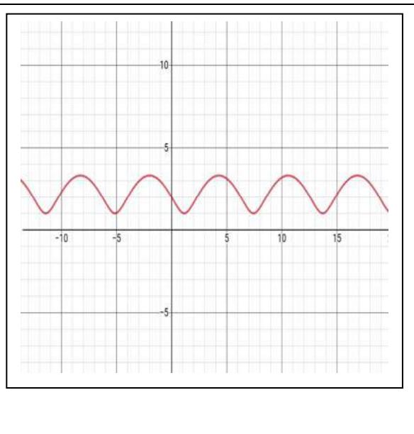Figure 2: Graphical representation of imaginary part of space dependent on energy based on equation (76)

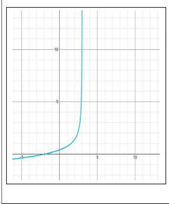Figure 4: Graphical representation of imaginary part of space dependent on time, based on equation (76)

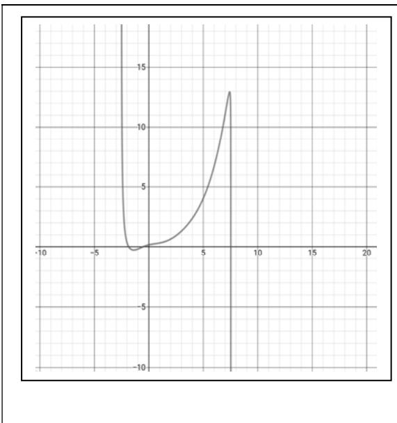Figure 5: Graphical representation of the real part of speed dependent on energy based on equation (77)

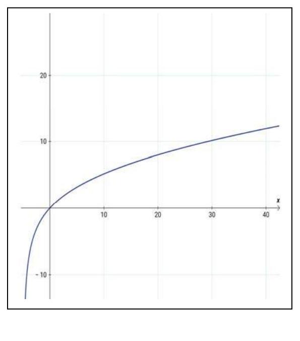Figure 7: Graphical representation of the real part of speed dependent on time, based on equation (77)

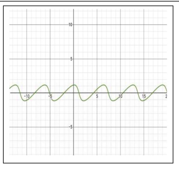Figure 6: Graphical representation of imaginary part of speed dependent on energy based on equation (78)

In addition to the above, the results of the generic equations are presented here below:

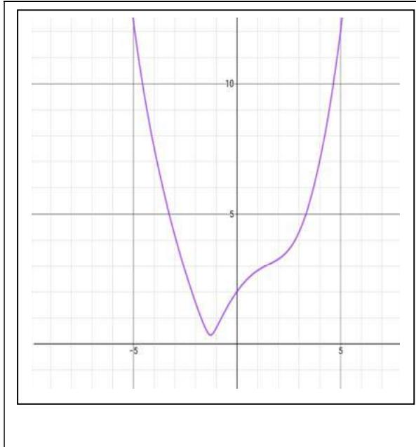Figure 9: Graphical representation of generic real part of space dependent on time, based on equation (79)

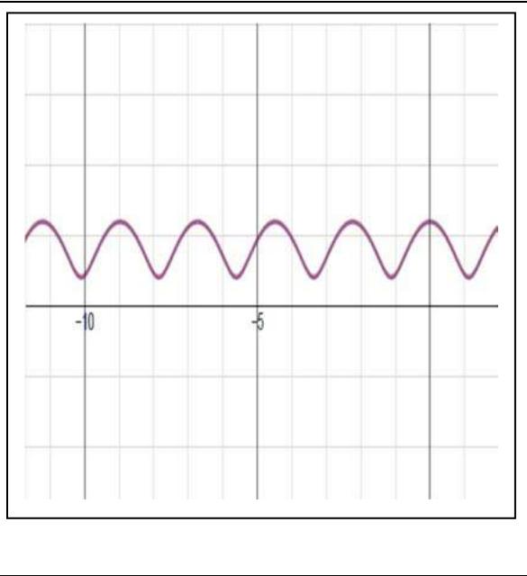Figure 8: Graphical representation of imaginary part of speed dependent on time, based on equation (78)

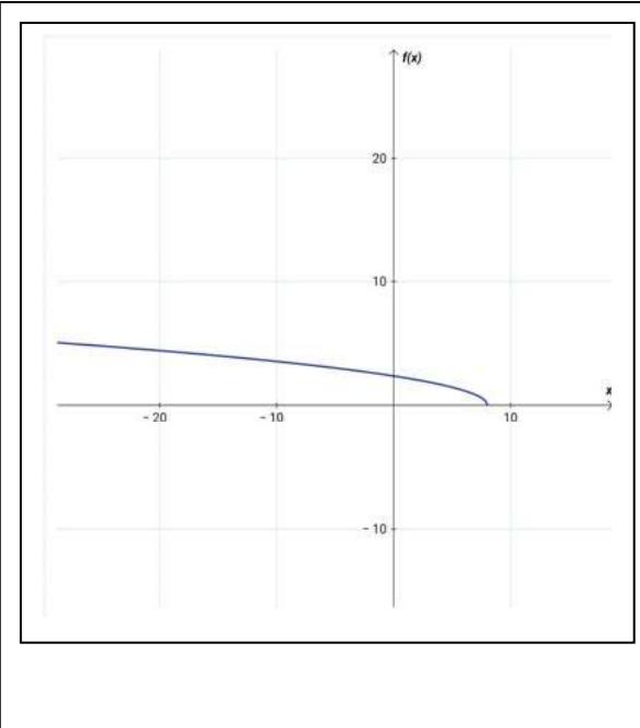Figure 11: Graphical representation of generic real part of space dependent on energy based on equation (79)

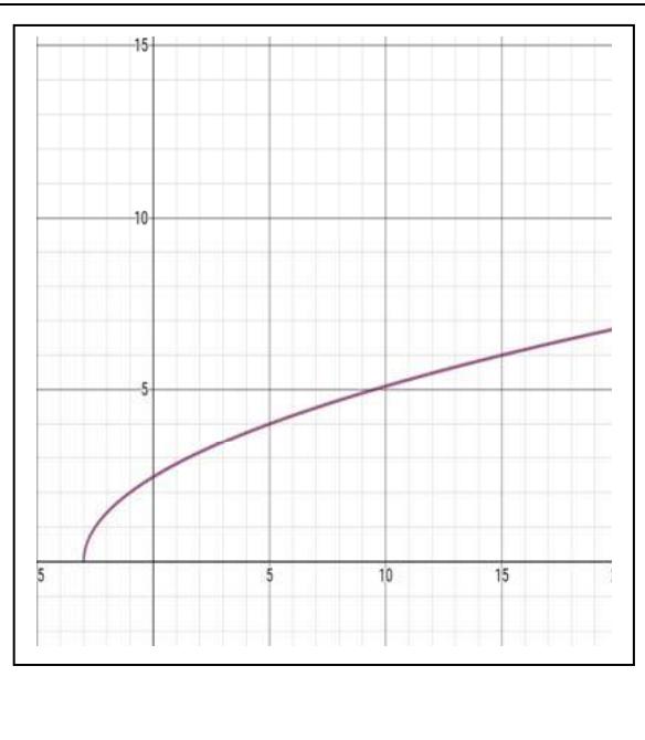Figure 10: Graphical representation of generic imaginary part of space dependent on time, based on equation (82)

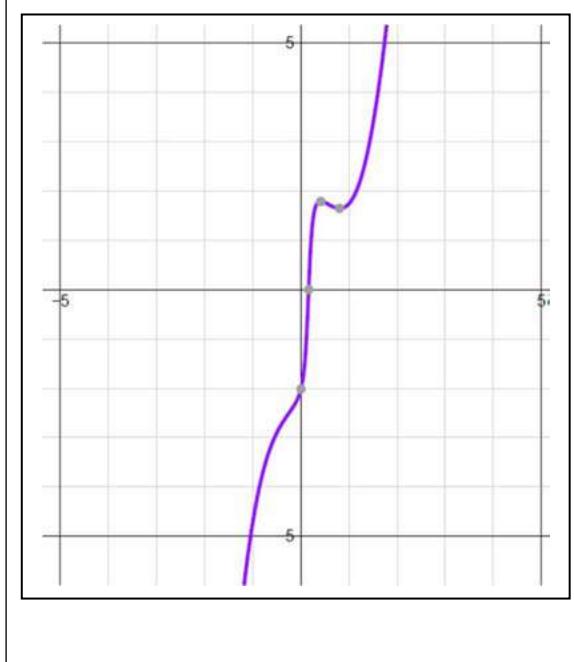Figure 13: Graphical representation of generic real part of speed dependent on time, based on equation (86)

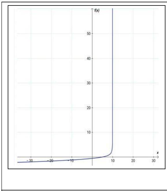Figure 15: Graphical representation of generic real part of speed dependent on energy based on equation (86)

{"image_source":{"path":"images/27b40756cd4901daee3af46900aa7fdf67b39d545e7a48e5b9b07de4aa650f66.jpg"},"content":"","chart_caption":[],"chart_footnote":[]}

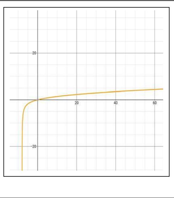Figure 14: Graphical representation of generic imaginary part of speed dependent on time, based on equation (84)

The equations developed reveal that space and speed are interconnected with both energy and time. To investigate how space and speed change simultaneously with respect to energy and time, the following three-dimensional graphs have been developed, assigning energy to the x-axis and time to the y-axis. In all these graphs, time has been considered to be equal to or greater than zero ( ) based on the causational law.

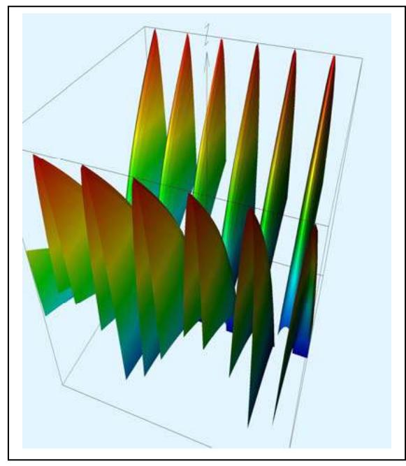Figure 12: Graphical representation of generic imaginary part of space dependent on energy based on equation (82)

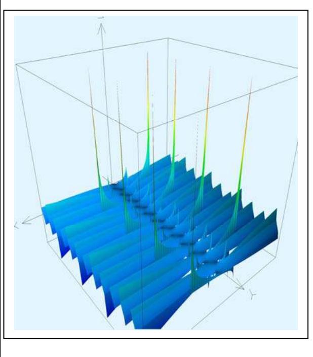Figure 17: 3-dimensional representation of equation (76)

{"image_source":{"path":"images/f5ef2cf8b956c1fd540a6436bae9122eb0fe3aad3ae67a1d5c482b211b5f515a.jpg"},"content":"","chart_caption":[],"chart_footnote":[]} {"image_source":{"path":"images/a16c42e1e04d589b5344409dd4f99c5ff859a8ab4c82baa97bbf8c85427a93b4.jpg"},"content":"","chart_caption":[{"type":"text","content":"Figure 19: 3-dimensional representation of equation (75)"},{"type":"text","content":"Figure 18: 3-dimensional representation of equation (78)"},{"type":"text","content":"Figure 20: 3-dimensional representation of equation (77)"}],"chart_footnote":[]}

{"image_source":{"path":"images/bd976239f412aae6b46e60954388011f63dfab81a5614892a7247962e27e7efb.jpg"},"content":"","chart_caption":[{"type":"text","content":"Figure 21: 3-dimensional representation of equation (82)"}],"chart_footnote":[]} {"image_source":{"path":"images/52970d29f443f73973636e955a4c3aba10db1d68d1f725c2c84c50d4aa3e6116.jpg"},"content":"","chart_caption":[{"type":"text","content":"Figure 22: 3-dimensional representation of equation (84)"}],"chart_footnote":[]}

{"image_source":{"path":"images/b6cdc36ceebe40118f619a47b2aa785d9ff60eecdf62ec73a415a28da76d70ed.jpg"},"content":"","chart_caption":[{"type":"text","content":"Figure 23: 3-dimensional representation of equation (79)"}],"chart_footnote":[]} {"image_source":{"path":"images/92d0237e116db087d7ec42d484e4cb080041da7efe97dce15a9395380b3f3b9d.jpg"},"content":"","chart_caption":[],"chart_footnote":[{"type":"text","content":"Figure 24: 3-dimensional representation of equation (86)"}]}

The analysis of the constraints that are described in equations (56), (59), (57), (61), (63), (65), (66), and (68) applies to the pem, whereas for a formed mass the relevant equations include (80), (81), (83), (86) and (87). The equations that satisfy all the constraints are equations (61), (63), (68) and (87). The following figures represent equations (61), (63) and (68).

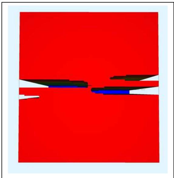Figure 16: Graphical representation of generic imaginary part of speed dependent on energy based on equation (84)

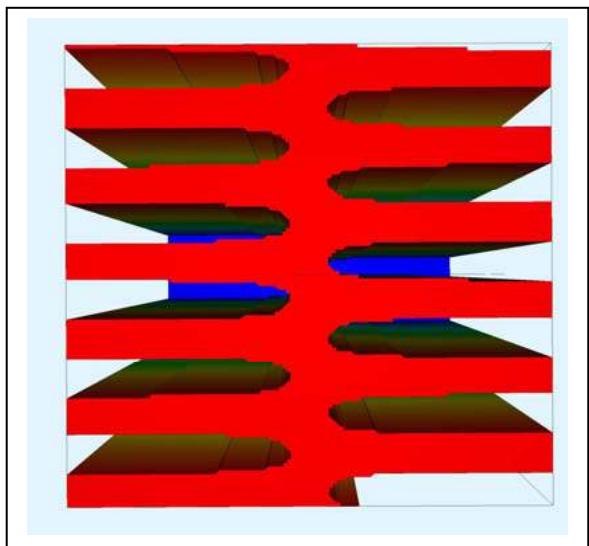Figure 25: E-t plane that equation (61) is valid Figure 26: E-t plane that equation (63) is valid

{"image_source":{"path":"images/5a84437ed6e9ad30f8a2a8af3f5102890b92319a81cd95d191814c8749a84d87.jpg"},"content":"","chart_caption":[{"type":"text","content":"Figure 27: E-t plane that equation (68) is valid"}],"chart_footnote":[]}

The areas presented in these graphs indicate the areas where the equations yield real solutions. However, special emphasis must be given to the boundary lines separating the areas where equations are valid (red-colored areas) from those where the equations are invalid (blue-colored areas). The pairs of values of energy and time on these boundary lines correspond to points where denominators attain the level of zero, leading the equations that express speed to incline towards infinity. As is expected, if mass reaches the limit values of these constraints, it can maximize the speed and consequently minimize the space.

{"image_source":{"path":"images/7151fe199d8a91a9cc9b2da5fa8f6ffcc20f517bbe8d6cf1c6988cac7e4a0487.jpg"},"content":"","chart_caption":[{"type":"text","content":"Figure 28: Representation of equation (88) speed vs energy"}],"chart_footnote":[]}

Equation (50) by the use of equation (72) turns into:

k _ {E} \gamma c ^ {2} = - \omega^ {2} \mathrm{e} ^ {\mathrm{i} (\omega t + \theta)} x _ {i} ^ {2} + 4 \mathrm{i} \omega \mathrm{e} ^ {\mathrm{i} (\omega t + \theta)} x _ {i} \cdot (\dot {x _ {\iota}}) + 2 \mathrm{e} ^ {\mathrm{i} (\omega t + \theta)} (x _ {i} \cdot (\ddot {x _ {\iota}}) + (\dot {x _ {\iota}}) ^ {2})\tag{89}

k _ {E} \gamma c ^ {2} \mathrm{e} ^ {\mathrm{i} (- (\omega t + \theta))} = - \omega^ {2} x _ {i} ^ {2} + 4 \mathrm{i} \omega x _ {i} \cdot (\dot {x _ {i}}) + 2 (x _ {i} \cdot (\ddot {x _ {i}}) + (\dot {x _ {i}}) ^ {2})\tag{90}

If the parameter is considered as a constant dependent on speed then (90) turns into:

Real Part:

k _ {E} \gamma c ^ {2} \mathrm{cos} (- (\omega t + \theta)) = - \omega^ {2} x _ {i} ^ {2} + 2 x _ {i} \cdot (\ddot {x _ {l}}) + 2 (\dot {x _ {l}}) ^ {2}\tag{91}

Imaginary Part:

k _ {E} \gamma c ^ {2} \sin (- (\omega t + \theta)) = 4 \omega x _ {i} \cdot (\dot {x _ {l}})\tag{92}

In addition, equation (52), with the use of equation (73), turns into:

(1 - k _ {E}) \gamma c ^ {2} = - 2 \omega^ {2} C _ {1} ^ {\prime} \mathrm{e} ^ {\mathrm{i} (\omega t _ {1} + \theta)} x _ {i} \cdot (\dot {x _ {l}}) - 2 \omega^ {2} (C _ {1} ^ {\prime} t + C _ {2} ^ {\prime}) \mathrm{e} ^ {\mathrm{i} (\omega t _ {1} + \theta)} \big (x _ {i} \cdot (\ddot {x _ {l}}) + (\dot {x _ {l}}) ^ {2} \big)\tag{93}

or

- \frac {(1 - k _ {E}) \gamma c ^ {2}}{2 \omega^ {2}} \mathrm{e} ^ {\mathrm{i} \left(- (\omega t _ {1} + \theta)\right)} = C _ {1} ^ {\prime} x _ {i} \cdot (\dot {x _ {\iota}}) + (C _ {1} ^ {\prime} t + C _ {2} ^ {\prime}) \big (x _ {i} \cdot (\ddot {x _ {\iota}}) + (\dot {x _ {\iota}}) ^ {2} \big)\tag{94}

The real and imaginary parts of which are:

Real part:

- \frac {(1 - k _ {E}) c ^ {2}}{2 \omega^ {2}} \gamma \mathrm{cos} (- (\omega t _ {1} + \theta)) = \Big (C _ {1} ^ {\prime} x _ {i} \cdot (\dot {x _ {\iota}}) + (C _ {1} ^ {\prime} t + C _ {2} ^ {\prime}) \big (x _ {i} \cdot (\ddot {x _ {\iota}}) + (\dot {x _ {\iota}}) ^ {2} \big) \Big)\tag{95}

Imaginary part:

- \frac {(1 - k _ {E}) c ^ {2}}{2 \omega^ {2}} \gamma \sin (- (\omega t _ {1} + \theta)) = 0\tag{96}

Finally, equation (44) turns into:

\gamma c ^ {2} = (i \ddot {\vartheta} - \dot {\vartheta} ^ {2}) e ^ {i \vartheta} x _ {i} ^ {2} + 4 i \dot {\vartheta} x _ {i} \cdot (\dot {x _ {l}}) e ^ {i \vartheta} + 2 (x _ {i} \cdot (\ddot {x _ {l}}) + (\dot {x _ {l}}) ^ {2}) e ^ {i \vartheta}\tag{97}

or

\gamma c ^ {2} e ^ {- i} = (i \ddot {\vartheta} - \dot {\vartheta} ^ {2}) x _ {i} ^ {2} + 4 i \dot {\vartheta} x _ {i} \cdot (\dot {x _ {l}}) + 2 \big (x _ {i} \cdot (\ddot {x _ {l}}) + (\dot {x _ {l}}) ^ {2} \big)\tag{98}

provided that:

m _ {0} = m _ {T}\tag{99}

m _ {0} = \mathbf {g} _ {\varepsilon} \mathbf {g} _ {\mathrm{t}} \mathbf {g} _ {\vec {s}} ^ {\prime}\tag{100}

Equation (94) is separated to real and imaginary parts as follows:

Real Part:

\gamma c ^ {2} \cos (- \vartheta) = - \dot {\vartheta} ^ {2} x _ {i} ^ {2} + 2 x _ {i} \cdot (\ddot {x _ {l}}) + 2 (\dot {x _ {l}}) ^ {2}\tag{101}

Imaginary Part:

\gamma c ^ {2} \sin (- \vartheta) = \ddot {\vartheta} x _ {i} ^ {2} + 4 \dot {\vartheta} x _ {i} \cdot (\dot {x _ {l}})\tag{102}

In all equations of this section the common characteristic is the lack of energy and mass from any part. This means that the solution of the differential equations relates space with time.

considering and that the calculations are carried out on axis i.

The solution of the equations (83), (84) and (95) are as follows:

\mathrm{x} _ {i, R e} (\mathrm{E}, \mathrm{t}) = \pm \frac {\sqrt {- k _ {E} \frac {c ^ {3}}{\sqrt {c ^ {2} - u ^ {2}}} \cos (\omega t + \theta) + \mathrm{k} _ {1} \omega \mathrm{e} ^ {\omega t} + \mathrm{k} _ {2} \omega^ {2} \mathrm{e} ^ {- \omega t}}}{\sqrt {2} \omega}\tag{103}

For the imaginary part:

x _ {i, I m} (u, t) = \pm \frac {\sqrt {k _ {E} \frac {c ^ {3}}{\sqrt {c ^ {2} - u ^ {2}}} \cos (\omega t + \theta) + k _ {3} \omega^ {2}}}{\sqrt {2} \omega}\tag{104}

= \pm \frac {\sqrt {- \frac {(1 - k _ {E})}{2 \omega^ {2}} \frac {c ^ {3}}{\sqrt {c ^ {2} - u ^ {2}}} c o s (\omega t _ {1} + \theta) \big (C _ {1} ^ {\prime 2} t ^ {2} + C _ {1} ^ {\prime} C _ {2} ^ {\prime} t + C _ {2} ^ {\prime 2} \big) + k _ {4} C _ {1} ^ {\prime} + 2 k _ {5} C _ {1} ^ {\prime 2} (C _ {2} ^ {\prime} t + C _ {2} ^ {\prime})}}{C _ {1} ^ {\prime} \sqrt {(C _ {1} ^ {\prime} t + C _ {2} ^ {\prime})}}\tag{105}

The combination of the equations (103) and (105) provide:

\begin{array}{l} \mathrm{x} _ {i, R e} (\mathrm{u}, \mathrm{t}) \\= \pm \frac {\sqrt {- k _ {E} \frac {c ^ {3}}{\sqrt {c ^ {2} - u ^ {2}}} \cos (\omega t + \theta) + k _ {1} \omega e ^ {\omega t} + k _ {2} \omega^ {2} e ^ {- \omega t}}}{\sqrt {2} \omega} \\\pm \frac {\sqrt {- \frac {(1 - k _ {E})}{2 \omega^ {2}} \frac {c ^ {3}}{\sqrt {c ^ {2} - u ^ {2}}} c o s (\omega t _ {1} + \theta) (C _ {1} ^ {\prime 2} t ^ {2} + C _ {1} ^ {\prime} C _ {2} ^ {\prime} t + C _ {2} ^ {\prime 2}) + k _ {4} C _ {1} ^ {\prime} + 2 k _ {5} C _ {1} ^ {\prime 2} (C _ {2} ^ {\prime} t + C _ {2} ^ {\prime})}}{C _ {1} ^ {\prime} \sqrt {(C _ {1} ^ {\prime} t + C _ {2} ^ {\prime})}} \end{array}\tag{106}

Which expresses the real part of space connected to time and speed, considering as:

\gamma = \frac {c}{\sqrt {c ^ {2} - u ^ {2}}}\tag{107}

The solution of (97) and (98), provide the following solutions:

\mathrm{x} _ {i, R e} (\mathrm{u}, \mathrm{t}) = \pm \frac {\sqrt {- \frac {c ^ {3}}{\sqrt {c ^ {2} - u ^ {2}}} \cos (p _ {1} t + p _ {2}) + p _ {3} p _ {1} \mathrm{e} ^ {p _ {1} \mathrm{t}} + p _ {4} p _ {1} ^ {2} \mathrm{e} ^ {- p _ {1} \mathrm{t}}}}{\sqrt {2} p _ {1}}\tag{108}

and

x _ {i, I m} (u, t) = \pm \frac {\sqrt {\frac {c ^ {3}}{\sqrt {c ^ {2} - u ^ {2}}} \cos (p _ {1} t + p _ {2}) + p _ {5} p _ {1} ^ {2}}}{\sqrt {2} p _ {1}}\tag{109}

considering:

It is noticed that in equations (103), (104) and (105) the time and space are connected directly without the use of energy or mass, but this is expected since the total energy of the mass has been replaced by the equation (47).

IV. DISCUSSION

The equations that have been developed so far indicate that space and speed are functions of energy and time. The behavior of space and speed are analyzed in a mathematical way, producing corresponding equation, followed by a comparison of the dependence on energy, since the equations developed indicate a direct relation between these three quantities. Equations deriving from the relativistic expression of energy are used to carry out a complete investigation that includes speed.

4.1 Analysis of the Speed Equations

This paragraph examines the equations of speed deriving from equation (38), which is expressed in the set of complex numbers, starting with those that are described by the imaginary part this equation. The analysis describes the change and possible limitations of speed related to energy and compares the equation with the basic expression of speed, as expressed in equation (2), and expands to the use of the relativistic models and equations.

4.1.1 The Analysis of the Imaginary Part of the Speed Equations

The widely used expression of kinetic energy is , so the expression of speed depending on energy is:

u = \pm \sqrt {\frac {2 E _ {k}}{m}}, m \neq 0\tag{110}

The study of equation (45), depending on energy, reveals a similarity to the equation

f (y) = k _ {y} \sqrt {y}\tag{111}

with , given a specific value of time. This is the same format that aligns with equation (110). The difference between (78) and the speed equation (110) lies in the term and the trigonometric terms. In the case where the factor is equal to zero, i.e., , it receives the format as follows:

\dot {x} (\mathrm{E}) = \sqrt {\frac {k _ {E} \mathrm{E}}{\mu_ {0}} \cos (\omega t + \theta)} \cdot \tan (\omega t + \theta)\tag{112}

This format is of the same type as equation (110) or (111), considering a specific value of time. Another difference between equations (78) and (110) is that equation (110) does not mention any explicit reference to time, which is why equation (78) is considered more comprehensive. The restrictions that apply to equation (78) are:

\frac {k _ {E} \mathrm{E}}{\mu_ {0}} \cos (\omega t + \theta) + \mathrm{k} _ {3} \omega^ {2} > 0\tag{113}

Finally, equation (110) shares structural similarities with (78) and (84), which means that both (78) and (84) express speed in an expanded way compared to the typical expression of speed, depending on energy. Notably, both these equations are the results of the solution of the imaginary components of (38) and (44), respectively. Figure 29 shows the representation of (78), (84), and (110) in graphical format. The same figure also includes the representation of equation (88) which represents the change of speed over the relativistic total energy.

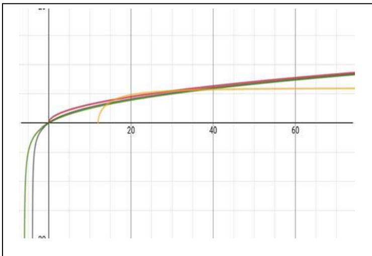Figure 29: Graphical presentation of equations (78), (84), (88) and (110)

Black line presents equation (78)

Green line presents equation (84)

Yellow line represents equation (88)

Red line presents equation (100) While investigating the potential limitations of speed, it is important to find the limit of these equations as energy moves to infinity. In such a case, the limit of (78) as energy tends towards infinity is:

\lim _ {E \to + \infty} \dot {x} (t) = \lim _ {E \to + \infty} \frac {\frac {\mathrm{E}}{\mu_ {0}} \sin (\omega t + \theta)}{2 \sqrt {\frac {\mathrm{E}}{\mu_ {0}} \cos (\omega t + \theta) + \mathrm{k} _ {3} \omega^ {2}}}\tag{114}

or

\lim _ {E \to + \infty} \dot {x} (t) = \lim _ {E \to + \infty} \frac {\frac {\mathrm{E}}{\mu_ {0}} \sin (\omega t + \theta) \sqrt {\frac {\mathrm{E}}{\mu_ {0}} \cos (\omega t + \theta) + k _ {3} \omega^ {2}}}{2 \left(\frac {\mathrm{E}}{\mu_ {0}} \cos (\omega t + \theta) + k _ {3} \omega^ {2}\right)} = \infty\tag{115}

In addition, the limit of (84) as energy tends towards infinity is:

\lim _ {E \to + \infty} \dot {x} (t) = \lim _ {E \to + \infty} \frac {\frac {E}{m _ {0 T}} \sin (p _ {1} t + p _ {2})}{2 \sqrt {\frac {E}{m _ {0 T}} \cos (p _ {1} t + p _ {2}) + p _ {5} p _ {1} ^ {2}}} = \infty\tag{116}

The outcome of this analysis is that, considering only these equations, there is no apparent limitation for the value of speed, as energy tends to infinity.

On the other hand, a certain combination of values of time and energy may lead the denominator in these equations to approach zero, i.e.:

\frac {E _ {1}}{m _ {0 T}} c o s (p _ {1} t _ {1} + p _ {2}) + p _ {5} p _ {1} ^ {2} = 0\tag{117}

wherein the speed tends to infinity, i.e.

\lim _ {E \to E _ {1}} \frac {\frac {\mathrm{E}}{\mu_ {0}} \sin (\omega t _ {1} + \theta)}{2 \sqrt {\frac {\mathrm{E}}{\mu_ {0}} \cos (\omega t _ {1} + \theta) + k _ {3} \omega^ {2}}} = \infty\tag{118}

However, this pair of values does not affect the format of equations (78), (84), and (110) expressed in graphs, as energy tends to infinity.

The use of relativistic mechanics describes the total energy of a mass by the relation (47) whereas the speed, if calculated from this model, results in equation (110).

Of course, in relativistic mechanics, it is taken axiomatically that the maximum speed a mass can reach is that of light (c) which is also objective for all bodies [20], [21], [22].

If we compare the relations (110) and the relation (111) with the relations (782) and (82) which results from the analysis of the imaginary part of the energy, similarities are observed. The expression of the speed through the relation (88) shows the limit set by the relative axiom. Although the equations (78), (84) and (110) show that the speed does not tend to some given value, the axiom of relativistic mechanics could also apply in the case of the imaginary part of this model.

4.1.2 Analysis of the Real Part of Speed - Differentiation towards other Models

The two models of classical and relativistic physics, consider mass as a given state. The differentiation of this work lies in the consideration of mass as a dynamic quantity. The result of this differentiation in combination with the expression of mass through the wide magnitude of complex numbers allows the expression of velocity with an additional term, shown in the relations (78) and (84). Therefore, if it is assumed that the limitation of velocity to the speed of light applies to the expression of the imaginary part in the relations (78) and (84), in the real part this does not seem to have any effect, as shown in the relations (77) and (79).

Equations (75) and (86), depending on energy, as presented in Figure 1 and Figure 15, respectively, reveal a value of energy specific for each equation, which, when attained, mass can travel at infinite speed, given a specific time value. This can be expressed for equation (108) as follows:

\lim _ {E \to E _ {l}} \dot {x} _ {i, R e} (t) = \lim _ {E \to E _ {l}} \frac {\frac {E}{m _ {0 T}} \sin (p _ {1} t _ {1} + p _ {2}) + p _ {3} p _ {1} \mathrm{e} ^ {p t _ {1}} - p _ {4} p _ {1} ^ {2} \mathrm{e} ^ {- p _ {1} t _ {1}}}{2 \sqrt {2} \sqrt {- \frac {E}{m _ {0 T}} \cos (p _ {1} t _ {1} + p _ {2}) + p _ {3} p _ {1} \mathrm{e} ^ {p _ {1} t _ {1}} + p _ {4} p _ {1} ^ {2} \mathrm{e} ^ {- p _ {1} t _ {1}}}} = \infty\tag{119}

where is a specific time value, and is the value of energy that can zero the denominator, and when the energy approaches this value, then speed tends to infinity. This value can be calculated as follows:

- E _ {l} \frac {1}{m _ {0 T}} \cos (p _ {1} t _ {1} + p _ {2}) + p _ {3} p _ {1} \mathrm{e} ^ {p _ {1} t _ {1}} + p _ {4} p _ {1} ^ {2} \mathrm{e} ^ {- p _ {1} t _ {1}} = 0\tag{120}

or

E _ {l} = m _ {0 T} \frac {p _ {3} p _ {1} \mathrm{e} ^ {p _ {1} t _ {1}} + p _ {4} p _ {1} ^ {2} \mathrm{e} ^ {- p _ {1} t _ {1}}}{\cos (p _ {1} t _ {1} + p _ {2})}, \cos (p _ {1} t _ {1} + p _ {2}) \neq 0\tag{121}

This expression could lead to an investigation of the way in which energy could be distributed in the mass so that it moves at a speed, possibly, greater than that of light. An example is the division of total energy into energy and exergy. Also, in many systems there is active and inactive power. Correspondingly, further research could be done on something similar.

Another important outcome comes from the combination of equations (77) with (78) and (88) or (84) with (86) and (88). The combination of equations (84), (86) and (88) is presented in Figure 30, suggesting that given the similarity of (78) to (110), the mass would typically move according to equation (78) under standard conditions. However, if the mass factors are modified, mass can move from equation (84) to equation (86), which means that mass can start traveling in the way already known but, with the appropriate values of factors, can move to equation (86) line and when to receive the required amount of energy, travel at infinite speed. In addition, even considering the movement of a mass based on (88) again, it can be concluded that, if the factors of mass are correctly selected, then mass can move to the line of equation (86) and travel with infinite speed.

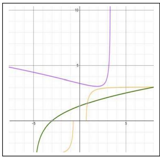Figure 30: Graphing representation of equations (84) (green line), (86) (purple line) and (88) (yellow line)

In addition, if this combination of energy and time is inserted into equations (77) and (86), space collapses to zero. This is made apparent in the combination of Figure 1 and Figure 6, as well as Figure 13 and Figure 17. The interpretation of this combination of energy and time is that when mass receives a critical amount of energy, it can travel with infinite speed, minimizing space to zero. This condition is done at a specific value of energy which is common for speed and space, as presented in Figure 31.

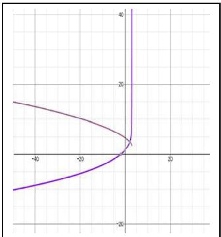Figure 31: Representation of equation (75) of space and (77) of speed in the same plane

4.2 Analysis of Equations Comparing to Time Parameter

The comparison of the equations (104) and (106) with equation (75) and (76) of the pem as well as the equations (108) and (109) with equations (79) and (82) of the generic model it is noticed that the results are similar in relation to time. Furthermore, the same outcome results from the comparison of the graphs that are produced from these equations. The equations (77), (78), (79) and (84) that express speed, are produced only for the equations of the expanded energy model.

This result is expected since the factors that are included in the equations derive from the equation:

\frac {\mathrm{E}}{\mathrm{m} _ {0}} = \gamma c ^ {2}\tag{122}

Equation (73) that expresses space can be expressed in another format, i.e.:

\frac {E}{m _ {0 T}} = \frac {p _ {1} ^ {2} (2 x _ {i , I m} ^ {2} - p _ {5})}{\cos (p _ {1} t + p _ {2})}\tag{123}

The implementation of equation (122) to equation (123) turns the latter to:

\gamma c ^ {2} = \frac {p _ {1} ^ {2} (2 x _ {i , I m} ^ {2} - p _ {5})}{\cos (p _ {1} t + p _ {2})}\tag{124}

which relation indicates a relation between space and time. Similar equations can be developed for all other expressions of space. This ascertainment proves that indeed there is a relation between space and time with energy.

Graphs obtained from imaginary components of pem and generic mass equations appear as trigonometric patterns. The graphical results from equations (77) and (82) demonstrate distinct variations which stem from their differing parameters. The speed equations obtained from the imaginary components of mathematics such as equations (67) and (84) present trigonometric behavior patterns. Equation (84) produces a complex graph through its multiple discontinuities that occur within brief intervals. The sophisticated nature of the created mass structure becomes apparent through this complexity.

Three-dimensional graphs generated from equations (75), (76), (77), and (78) for pem, as well as (79), (82), (84), and (86) for generic mass, illustrate changes in space or speed as functions of two variables: energy (E) on the x-axis and time (t) on the y-axis. The 3D graphs combine elements from two-dimensional energy-time plots to display information. The graph in Figure 24 presents speed changes alongside energy and time variations where speed rises with advancing energy and time. Equation (86) becomes invalid for specific pairings between energy and time since void regions emerge in the graph.

A comparison between pairs of pem and generic mass equations shows matching characteristics in their graphs. Equations (78) and (84) show equivalent behavior patterns through their appearance of space spikes at distinctive energy-time points. Equation (86) provides more continuous spatial outputs because the formed rigid mass structure hinders quick changes during energy and time operation. The graphical data in Figures 22 and 26 demonstrates that speed improves steadily as energy and time enlarge. The system shows undefined output regions when operating at low energy alongside low time values, yet these areas display unique patterns between pem and generic mass behavior. When chosen energy-time pairs are inserted into the mathematical equations, they produce results that lead to infinite speed.

4.3 Analysis of Space Equations in Relation to Factor y.

The comparison of equations (104) and (106) for pem, as well as (108) and (109) for the generic model, indicates a similarity with the equations (75) and (76) and also (79) and (82) that describe space with the expanded energy model. The difference between the two models is the use of the factor , which can be considered as a consequence of the equation (123).

On the other hand, the use of the factor, produces results that do not actually deviate from the initial relativistic expression of space. Taking as example equations (108) and (109), they can be expressed as:

\mathrm{x} _ {i, R e} (\mathrm{t}) = \pm \mathrm{c} \sqrt {\frac {1}{\sqrt {1 - \frac {u ^ {2}}{c ^ {2}}}}} \frac {\sqrt {- \cos (p _ {1} t + p _ {2}) + p _ {3} p _ {1} \mathrm{e} ^ {p _ {1} \mathrm{t}} + p _ {4} p _ {1} ^ {2} \mathrm{e} ^ {- p _ {1} \mathrm{t}}}}{\sqrt {2} p _ {1}}\tag{125}

and

x _ {i, I m} (t) = \pm c \sqrt {\frac {1}{\sqrt {1 - \frac {u ^ {2}}{c ^ {2}}}}} \frac {\sqrt {\cos (p _ {1} t + p _ {2}) + p _ {5} p _ {1} ^ {2}}}{\sqrt {2} p _ {1}}\tag{126}

which provide expressions between space and time. These expressions are not deviating from expressions that describe the way that space changes over speed , . The expressions are more generalised, but the format of change over the speed change is of the same type.

V. CONCLUSION

The expression of the energy obtained by a mass can be expanded if mass, either in the form of pem or in the more complicated format, is approached as a dynamic quantity. In this case space is related not only to time but energy as well, intruding a new comprehension of energy-space-time interactions. The expanded model of energy provides a wider expression of speed. The first expression approaches speed in a way that follows the limitations that are known to apply as the relativistic approach indicates. However, a different expression that arises, opens the option of mass, either in pem or complete format, to travel at speeds even higher than this of light, which is currently investigated at theoretical level, provided that the factors that express a mass are properly altered. Space, in this case, as expressed in the equations produced during the investigation, is minimized, tending to zero, as speed approaches infinite speed. What remains to be verified is the experimental and practical approach as to the speed a mass can reach, minimizing the space.

ACKNOWLEDGEMENTS

The author would like to extend his gratitude to the teams contributing to the development of ClassCalc software which has been used for the creation of the qualitative 2-dimensional graphs, the Surface Plotter 3D software which has proved invaluable in the creation of the 3-dimensional graphs and Wolfram alpha which facilitated the calculation of key parts of the derived equations.

− Conflict of Interest

The authors declare no conflict of interest.

− Ethical Approval

Not applicable

− Data Availability

The datasets used in this study are openly available at [repository link] and the source code is available on GitHub at [GitHub link].

− Funding

This work did not receive any external funding.

− References

17 Cites in Article

REFERENCE FORMAT

− Cite this article

Generating citation...

Classification
1

LCC Code: QC793.5.E425
Version of record

v1.0
Issue date

16 June 2025
Language

en

Download Article Access OJS

Open Access

Research Article

CC-BY-NC 4.0

Views 2.3K

Downloads 91

Year

Special Issue

Launch a focused special issue to highlight research, emerging trends, and expert insights in your academic field.

Keywords

12

Dynamic Mass Framework Energy Distribution High-Energy Physics Mass Factors Mass–Energy Interaction Point Energy Mass Relativity Theory Space–Time Dynamics Space–Time Relativistic Effects Superluminal Travel Theoretical Physics Time-Dependent Mass

A Dynamic Framework for Mass-Energy Interaction: Exploring the Role of Time and Relativity

IntelliPaper

− Abstract

− Explore Digital Article Text

I. INTRODUCTION

II. METHODOLOGY

2.1. analysis of the model

2.2 Relativistic Approach

B. Speed:

IV. DISCUSSION

4.1 Analysis of the Speed Equations

4.1.1 The Analysis of the Imaginary Part of the Speed Equations

4.1.2 Analysis of the Real Part of Speed - Differentiation towards other Models

4.2 Analysis of Equations Comparing to Time Parameter

V. CONCLUSION

ACKNOWLEDGEMENTS

− Conflict of Interest

− Ethical Approval

− Data Availability

− Funding

− References

− Cite this article

Classification

Version of record

Issue date

Language

Special Issue

Keywords

Next Research

Copy of Cardiovascular Risk Factors and Cardiovascular Risk in People Living with HIV: Comparison of Four Cardiovascular Risk Prediction Algorithms

Privacy preferences

A Dynamic Framework for Mass-Energy Interaction: Exploring the Role of Time and Relativity

IntelliPaper

Request Review Access

Order Article Reprints

− Abstract

− Explore Digital Article Text

I. INTRODUCTION

II. METHODOLOGY

2.1. analysis of the model

2.2 Relativistic Approach

3.1 Analysis of the Results basis the Expanded Energy Modal

B. Speed:

IV. DISCUSSION

4.1 Analysis of the Speed Equations

4.1.1 The Analysis of the Imaginary Part of the Speed Equations

4.1.2 Analysis of the Real Part of Speed - Differentiation towards other Models

4.2 Analysis of Equations Comparing to Time Parameter

V. CONCLUSION

ACKNOWLEDGEMENTS

− Conflict of Interest

− Ethical Approval

− Data Availability

− Funding

− References

− Cite this article

− Related Research

Classification

Version of record

Issue date

Language

Special Issue

Keywords

Next Research

Copy of Cardiovascular Risk Factors and Cardiovascular Risk in People Living with HIV: Comparison of Four Cardiovascular Risk Prediction Algorithms

Privacy preferences