Possible Relationship between Sea Quarks Distribution Functions and Valence Distribution Functions in Proton

# Introduction After Gell-Mann succeeded to predict the existence of $\Omega ^ { - }$ by estimating its mass by his eight-fold way model \[1\], people had believed that baryons including nucleons are consisted by three quarks. However, New Muon Collaboration (NMC) \[2\], NA51 Collaboration \[3\] and E866 Collaboration \[4\] reported $\bar { d } ^ { - } \bar { u }$ asymmetry in proton. These results has stimulated people’s concern for the structure of proton. As results, H1 and Zeus (DESY) \[5\] and Atlas (CERN) \[6\] have reported sea quarks (quark-antiquark system) distribution functions, valence quark distribution functions and gluon distribution functions in proton. These results show that proton has more profound structure than that composed by simple three quarks. H1 and Zeus results are obtained by electron-proton collision, while Atlas results are obtained by proton-proton collision. Especially, Atlas results show the following very interesting properties. Besides they found ss sea quarks distribution functions denoted as $\mathrm { x } \bar { s }$ , $\mathrm { x } \bar { d }$ value at $\mathbf { x } = 1 \times 1 0 ^ { - 3 }$ looks like equal to the peak value of $\cdot$ and $\mathrm { x } \bar { u }$ value at $\mathbf { x } = 1 \times 1 0 ^ { - 3 }$ looks like one half of the peak value of xu. In addition, $\cdot$ value at $\mathbf { x } = 1 \times 1 0 ^ { - 3 }$ looks like equal to $\cdot$ value at $\mathbf { x } = 1 \times 1 0 ^ { - 3 }$ . Note that Atlas group denote each sea quarks distribution functions as xu,xd and xs, respectively, and also denote valence u quark and valence d quark distribution functions as xu and xd, respectively \[6\]. These properties indicate that it is possible or rather probable that there are some relationship between sea quarks distribution functions and valence quark distribution functions. In this paper, we attempt to show behavior of $\bar { u }$ and $\bar { d }$ sea quarks distribution functions and that of valence u quark and valence d quark distribution functions starting from our charged pion distribution amplitude and functions shown in ref. \[7\] and ref. \[8\], respectively. # Formulation We proposed for description of baryons as composition of bound and unbound state of sea quarks \[9\]. By following those descriptions, proton is described as composition of a charged pion $\pi ^ { + } ( u \bar { d } )$ and a neutral pionπ° (mix of u and dd $( ( u \bar { u } - d \bar { d } ) / \sqrt { 2 } ) )$ besides s unbound sea quarks. Important point is that $\pi ^ { + }$ and $\pi ^ { 0 }$ can take either bound state or unbound state repeatedly. For an example of numerical calculation, we showed proton and neutron electromagnetic form factors using pion pair consideration \[10\]. Note that we used $\pi ^ { + }$ wave function for $\pi ^ { 0 }$ wave function in proton case in that paper because we had not obtained $\pi ^ { 0 }$ wave function yet at that paper’s publication date. In addition, we obtained a charged pion distribution amplitude \[7\] and its distribution function \[8\]. Using those arguments, we attempt to explain the behavior of Atlas experiment results \[6\]. Although we proposed that proton is composed as $\pi ^ { + }$ and $\pi ^ { 0 }$ besides $\mathsf { s } \bar { \boldsymbol { s } }$ in ref. \[9\], in reality, the distribution functions of $\mathrm { u } \bar { d }$ , uu and ${ \mathrm { d } } { \bar { d } }$ should be slightly different from those of $\pi ^ { + }$ and $\pi ^ { 0 }$ because there is no evidence that shows to exist exact $\pi ^ { + }$ and $\pi ^ { 0 }$ in proton. Thus, we use our distribution amplitude and functions of charged pion as basic forms but we deviate slightly to describe the distribution amplitude and functions of $\mathbf { u } \bar { d }$ , $\mathrm { u } \bar { u }$ and ${ \mathrm { d } } { \bar { d } }$ in proton. Here, we use our approximate forms for distribution amplitude and functions of charged pion. Note that, as we mentioned in ref. \[7\], our approximate forms are sufficient to compare to other proposed distribution amplitude, thus, also to other proposed distribution functions from the definition as shown in later. Our approximate form of distribution amplitude of charged pion is described as \[7\] $$ F _ { 3 } ( x ) = { \frac { 1 - x } { x } } { \Biggl ( } 1 - e ^ { - \rho { \frac { x } { 1 - x } } } { \Biggl ( } s i n \left( \rho { \frac { x } { 1 - x } } \right) + c o s \left( \rho { \frac { x } { 1 - x } } \right) { \Biggr ) } { \Biggr ) } $$ where 1\] Note that $F _ { 3 } ( x )$ is actually $| F _ { 3 } ( x ) |$ . From Eq. (1), our approximate form of the charged pion distribution functions is described as \[8\] $$ f _ { 3 } ( x ) = c o n s t x | F _ { 3 } ( x ) | = c o n s t ( 1 - x ) \left( 1 - e ^ { - \rho \frac { x } { 1 - x } } \left( s i n \left( \rho \frac { x } { 1 - x } \right) + c o s \left( \rho \frac { x } { 1 - x } \right) \right) \right) $$ We consider that sea quarks states correspond to unbound state. Here, we define unbound state as follows: Definition: Unbound state is a state corresponding to a distribution amplitude, that is, exponential $e ^ { - \rho \frac { x } { 1 - x } }$ becomes negligibly smal because the coupling constant $g ^ { 2 }$ is sufficiently small. Thus, Eq. (1) gives our distribution amplitude of sea quarks $\bar { d }$ that come from $\pi ^ { + }$ as $$ F _ { 3 } ^ { s e a { \bar { d } } } ( x ) = { \frac { 1 - x } { x } } $$ Thus, our distribution functions of $\bar { d }$ become $$ f _ { \pi ^ { + } } ^ { s e a \bar { d } } ( x ) = c o n s t x F _ { 3 } ^ { s e a \bar { d } } ( x ) = c o n s t ( 1 - x ) $$ Notation of $f _ { \pi ^ { + } } ^ { s e a \bar { d } } ( x )$ means sea quarks $\bar { d }$ distribution functions come from $\pi ^ { + }$ . The behavior of $f _ { \pi ^ { + } } ^ { s e a \bar { d } } ( x )$ q litt ha th distribution functions $\mathrm { x } \bar { d }$ shown in Atlas experiment results \[6\]. Therefore, we deviate distribution amplitude slightly from Eq. (1). To achieve this purpose, we return to the exact form of our distribution amplitude shown in Eq. (40) in ref. \[7\] as: $$ F _ { 3 } ( \left| q \right| ) = \Gamma \left( 1 + \frac { i } { \pi } \right) e ^ { - i \frac { \pi } { 4 } } \frac { 1 } { \sqrt { \left| \alpha \right| } } \int _ { 0 } ^ { \infty } d z e x p \left( - \frac { \left| q \right| } { \sqrt { 2 \left| \alpha \right| } } z ( 1 - i ) \right) e ^ { \frac { 1 } { 4 } z ^ { 2 } } \left( \frac { 1 } { 2 } z \right) ^ { - \frac { 1 } { 2 } } W _ { - \frac { 1 } { 4 } - \frac { i } { \pi } , - \frac { 1 } { 4 } } \left( \frac { 1 } { 2 } z ^ { 2 } \right) $$ $$ - \Gamma \left( 1 - \frac { i } { \pi } \right) e ^ { - i \frac { \pi } { 4 } } \frac { 1 } { \sqrt { | \alpha | } } \int _ { 0 } ^ { \infty } d z e x p \left( - \frac { | q | } { \sqrt { 2 | \alpha | } } z ( 1 + i ) \right) e ^ { \frac { 1 } { 4 } z ^ { 2 } } \left( \frac { 1 } { 2 } z \right) ^ { \frac { 1 } { 2 } } W _ { - \frac { 1 } { 4 } + \frac { i } { \pi } , - \frac { 1 } { 4 } } \left( \frac { 1 } { 2 } z ^ { 2 } \right) $$ To evaluate the integral in Eq. (5), we again divide the integral as $\textstyle { \int _ { 0 } ^ { \infty } d z = \int _ { 0 } ^ { u } d z + \int _ { u } ^ { \infty } d z }$ and use the argument for large lql case shown in ref. \[7\]. Then, our distribution amplitude is represented by following equation. $$ F _ { 3 } ( \left| q \right| ) = \Gamma \left( 1 + \frac { i } { \pi } \right) e ^ { - i \frac { \pi } { 4 } } \frac { 1 } { \sqrt { \left| \alpha \right| } } \int _ { 0 } ^ { u } d z e x p \left( - \frac { \left| q \right| } { \sqrt { 2 \left| \alpha \right| } } z ( 1 - i ) \right) e ^ { \frac { 1 } { 4 } z ^ { 2 } } \left( \frac { 1 } { 2 } z \right) ^ { - \frac { 1 } { 2 } } W _ { - \frac { 1 } { 4 } \frac { i } { \pi } , \frac { 1 } { 4 } } \left( \frac { 1 } { 2 } z ^ { 2 } \right) $$ $$ - \Gamma \left( 1 - \frac { i } { \pi } \right) e ^ { - i \frac { \pi } { 4 } } \frac { 1 } { \sqrt { | \alpha | } } \int _ { 0 } ^ { u } d z e x p \left( - \frac { | q | } { \sqrt { 2 | \alpha | } } z ( 1 + i ) \right) e ^ { \frac { 1 } { 4 } z ^ { 2 } } \left( \frac { 1 } { 2 } z \right) ^ { - \frac { 1 } { 2 } } W _ { \frac { 1 } { 4 } + \frac { i } { \pi } , - \frac { 1 } { 4 } } \left( \frac { 1 } { 2 } z ^ { 2 } \right) $$ Recalling that we obtained our approximate form of pion distribution amplitude using only the first term of $M _ { \kappa , \mu } ( z )$ to evaluate the integral in the case of large $| q |$ and also recalling that $W _ { \kappa , \mu } ( z )$ is # Introduction After Gell-Mann succeeded to predict the existence of $\Omega ^ { - }$ by estimating its mass by his eight-fold way model \[1\], people had believed that baryons including nucleons are consisted by three quarks. However, New Muon Collaboration (NMC) \[2\], NA51 Collaboration \[3\] and E866 Collaboration \[4\] reported $\bar { d } ^ { - } \bar { u }$ asymmetry in proton. These results has stimulated people’s concern for the structure of proton. As results, H1 and Zeus (DESY) \[5\] and Atlas (CERN) \[6\] have reported sea quarks (quark-antiquark system) distribution functions, valence quark distribution functions and gluon distribution functions in proton. These results show that proton has more profound structure than that composed by simple three quarks. H1 and Zeus results are obtained by electron-proton collision, while Atlas results are obtained by proton-proton collision. Especially, Atlas results show the following very interesting properties. Besides they found ss sea quarks distribution functions denoted as $\mathrm { x } \bar { s }$ , $\mathrm { x } \bar { d }$ value at $\mathbf { x } = 1 \times 1 0 ^ { - 3 }$ looks like equal to the peak value of $\cdot$ and $\mathrm { x } \bar { u }$ value at $\mathbf { x } = 1 \times 1 0 ^ { - 3 }$ looks like one half of the peak value of xu. In addition, $\cdot$ value at $\mathbf { x } = 1 \times 1 0 ^ { - 3 }$ looks like equal to $\cdot$ value at $\mathbf { x } = 1 \times 1 0 ^ { - 3 }$ . Note that Atlas group denote each sea quarks distribution functions as xu,xd and xs, respectively, and also denote valence u quark and valence d quark distribution functions as xu and xd, respectively \[6\]. These properties indicate that it is possible or rather probable that there are some relationship between sea quarks distribution functions and valence quark distribution functions. In this paper, we attempt to show behavior of $\bar { u }$ and $\bar { d }$ sea quarks distribution functions and that of valence u quark and valence d quark distribution functions starting from our charged pion distribution amplitude and functions shown in ref. \[7\] and ref. \[8\], respectively. # Formulation We proposed for description of baryons as composition of bound and unbound state of sea quarks \[9\]. By following those descriptions, proton is described as composition of a charged pion $\pi ^ { + } ( u \bar { d } )$ and a neutral pionπ° (mix of u and dd $( ( u \bar { u } - d \bar { d } ) / \sqrt { 2 } ) )$ besides s unbound sea quarks. Important point is that $\pi ^ { + }$ and $\pi ^ { 0 }$ can take either bound state or unbound state repeatedly. For an example of numerical calculation, we showed proton and neutron electromagnetic form factors using pion pair consideration \[10\]. Note that we used $\pi ^ { + }$ wave function for $\pi ^ { 0 }$ wave function in proton case in that paper because we had not obtained $\pi ^ { 0 }$ wave function yet at that paper’s publication date. In addition, we obtained a charged pion distribution amplitude \[7\] and its distribution function \[8\]. Using those arguments, we attempt to explain the behavior of Atlas experiment results \[6\]. Although we proposed that proton is composed as $\pi ^ { + }$ and $\pi ^ { 0 }$ besides $\mathsf { s } \bar { \boldsymbol { s } }$ in ref. \[9\], in reality, the distribution functions of $\mathrm { u } \bar { d }$ , uu and ${ \mathrm { d } } { \bar { d } }$ should be slightly different from those of $\pi ^ { + }$ and $\pi ^ { 0 }$ because there is no evidence that shows to exist exact $\pi ^ { + }$ and $\pi ^ { 0 }$ in proton. Thus, we use our distribution amplitude and functions of charged pion as basic forms but we deviate slightly to describe the distribution amplitude and functions of $\mathbf { u } \bar { d }$ , $\mathrm { u } \bar { u }$ and ${ \mathrm { d } } { \bar { d } }$ in proton. Here, we use our approximate forms for distribution amplitude and functions of charged pion. Note that, as we mentioned in ref. \[7\], our approximate forms are sufficient to compare to other proposed distribution amplitude, thus, also to other proposed distribution functions from the definition as shown in later. Our approximate form of distribution amplitude of charged pion is described as \[7\] $$ F _ { 3 } ( x ) = { \frac { 1 - x } { x } } { \Biggl ( } 1 - e ^ { - \rho { \frac { x } { 1 - x } } } { \Biggl ( } s i n \left( \rho { \frac { x } { 1 - x } } \right) + c o s \left( \rho { \frac { x } { 1 - x } } \right) { \Biggr ) } { \Biggr ) } $$ where 1\] Note that $F _ { 3 } ( x )$ is actually $| F _ { 3 } ( x ) |$ . From Eq. (1), our approximate form of the charged pion distribution functions is described as \[8\] $$ f _ { 3 } ( x ) = c o n s t x | F _ { 3 } ( x ) | = c o n s t ( 1 - x ) \left( 1 - e ^ { - \rho \frac { x } { 1 - x } } \left( s i n \left( \rho \frac { x } { 1 - x } \right) + c o s \left( \rho \frac { x } { 1 - x } \right) \right) \right) $$ We consider that sea quarks states correspond to unbound state. Here, we define unbound state as follows: Definition: Unbound state is a state corresponding to a distribution amplitude, that is, exponential $e ^ { - \rho \frac { x } { 1 - x } }$ becomes negligibly smal because the coupling constant $g ^ { 2 }$ is sufficiently small. Thus, Eq. (1) gives our distribution amplitude of sea quarks $\bar { d }$ that come from $\pi ^ { + }$ as $$ F _ { 3 } ^ { s e a { \bar { d } } } ( x ) = { \frac { 1 - x } { x } } $$ Thus, our distribution functions of $\bar { d }$ become $$ f _ { \pi ^ { + } } ^ { s e a \bar { d } } ( x ) = c o n s t x F _ { 3 } ^ { s e a \bar { d } } ( x ) = c o n s t ( 1 - x ) $$ Notation of $f _ { \pi ^ { + } } ^ { s e a \bar { d } } ( x )$ means sea quarks $\bar { d }$ distribution functions come from $\pi ^ { + }$ . The behavior of $f _ { \pi ^ { + } } ^ { s e a \bar { d } } ( x )$ q litt ha th distribution functions $\mathrm { x } \bar { d }$ shown in Atlas experiment results \[6\]. Therefore, we deviate distribution amplitude slightly from Eq. (1). To achieve this purpose, we return to the exact form of our distribution amplitude shown in Eq. (40) in ref. \[7\] as: $$ F _ { 3 } ( \left| q \right| ) = \Gamma \left( 1 + \frac { i } { \pi } \right) e ^ { - i \frac { \pi } { 4 } } \frac { 1 } { \sqrt { \left| \alpha \right| } } \int _ { 0 } ^ { \infty } d z e x p \left( - \frac { \left| q \right| } { \sqrt { 2 \left| \alpha \right| } } z ( 1 - i ) \right) e ^ { \frac { 1 } { 4 } z ^ { 2 } } \left( \frac { 1 } { 2 } z \right) ^ { - \frac { 1 } { 2 } } W _ { - \frac { 1 } { 4 } - \frac { i } { \pi } , - \frac { 1 } { 4 } } \left( \frac { 1 } { 2 } z ^ { 2 } \right) $$ $$ - \Gamma \left( 1 - \frac { i } { \pi } \right) e ^ { - i \frac { \pi } { 4 } } \frac { 1 } { \sqrt { | \alpha | } } \int _ { 0 } ^ { \infty } d z e x p \left( - \frac { | q | } { \sqrt { 2 | \alpha | } } z ( 1 + i ) \right) e ^ { \frac { 1 } { 4 } z ^ { 2 } } \left( \frac { 1 } { 2 } z \right) ^ { \frac { 1 } { 2 } } W _ { - \frac { 1 } { 4 } + \frac { i } { \pi } , - \frac { 1 } { 4 } } \left( \frac { 1 } { 2 } z ^ { 2 } \right) $$ To evaluate the integral in Eq. (5), we again divide the integral as $\textstyle { \int _ { 0 } ^ { \infty } d z = \int _ { 0 } ^ { u } d z + \int _ { u } ^ { \infty } d z }$ and use the argument for large lql case shown in ref. \[7\]. Then, our distribution amplitude is represented by following equation. $$ F _ { 3 } ( \left| q \right| ) = \Gamma \left( 1 + \frac { i } { \pi } \right) e ^ { - i \frac { \pi } { 4 } } \frac { 1 } { \sqrt { \left| \alpha \right| } } \int _ { 0 } ^ { u } d z e x p \left( - \frac { \left| q \right| } { \sqrt { 2 \left| \alpha \right| } } z ( 1 - i ) \right) e ^ { \frac { 1 } { 4 } z ^ { 2 } } \left( \frac { 1 } { 2 } z \right) ^ { - \frac { 1 } { 2 } } W _ { - \frac { 1 } { 4 } \frac { i } { \pi } , \frac { 1 } { 4 } } \left( \frac { 1 } { 2 } z ^ { 2 } \right) $$ $$ - \Gamma \left( 1 - \frac { i } { \pi } \right) e ^ { - i \frac { \pi } { 4 } } \frac { 1 } { \sqrt { | \alpha | } } \int _ { 0 } ^ { u } d z e x p \left( - \frac { | q | } { \sqrt { 2 | \alpha | } } z ( 1 + i ) \right) e ^ { \frac { 1 } { 4 } z ^ { 2 } } \left( \frac { 1 } { 2 } z \right) ^ { - \frac { 1 } { 2 } } W _ { \frac { 1 } { 4 } + \frac { i } { \pi } , - \frac { 1 } { 4 } } \left( \frac { 1 } { 2 } z ^ { 2 } \right) $$ Recalling that we obtained our approximate form of pion distribution amplitude using only the first term of $M _ { \kappa , \mu } ( z )$ to evaluate the integral in the case of large $| q |$ and also recalling that $W _ { \kappa , \mu } ( z )$ is defined as \[1, a light deviation an be considered by adding the first term of $M _ { \kappa , - \mu } ( z )$ because actual form of $W _ { \kappa , \mu } ( z )$ in Eq. (6) is $W _ { \kappa , \mu } \left( \frac { 1 } { 2 } z ^ { 2 } \right)$ . The definition of $M _ { \kappa , \mu } ( z )$ is described as \[11\] $$ M _ { \kappa , \mu } ( z ) = z ^ { \mu + \frac { 1 } { 2 } } e ^ { - \frac { z } { 2 } } { } _ { 1 } F _ { 1 } \left( \mu - \kappa , 2 \mu + 1 ; z \right) $$ where ${ } _ { 1 } F _ { 1 }$ is the confluent hypergeometric series defined as \[11\] $$ { _ { 1 } F _ { 1 } } \left( \eta , \zeta ; z \right) = \sum _ { n = 0 } ^ { \infty } { \frac { \eta ( \eta + 1 ) \cdot \cdot \cdot \left( \eta + n - 1 \right) z ^ { n } } { \zeta ( \zeta + 1 ) \cdot \cdot \cdot \left( \zeta + n - 1 \right) } } = 1 + \sum _ { n = 1 } ^ { \infty } { \frac { \eta ( \eta + 1 ) \cdot \cdot \cdot \left( \eta + n - 1 \right) } { \zeta ( \zeta + 1 ) \cdot \cdot \cdot \left( \zeta + n - 1 \right) } } { \frac { z ^ { n } } { n ! } } $$ Thus, the first term of $M _ { \kappa , - \mu } \left( \frac { 1 } { 2 } z ^ { 2 } \right)$ in the case of and $\textstyle \mu = - { \frac { 1 } { 4 } }$ becomes Thus, Eq. (6) becomes $$ \begin{aligned} F _ { 3 } ( | q | ) & = e ^ { - i \frac { \pi } { 4 } } 2 ^ { \frac { 1 } { 4 } } \frac { 1 } { \sqrt { | \alpha | } } \int _ { 0 } ^ { u } d z \exp \left( - \frac { | q | } { \sqrt { 2 | \alpha | } } z ( 1 - i ) \right) \left[ \Gamma ( \frac { 1 } { 2 } ) + \frac { \Gamma ( 1 + \frac { i } { \pi } ) } { \Gamma ( \frac { 1 } { 2 } + \frac { i } { \pi } ) } \Gamma ( - \frac { 1 } { 2 } ) ( \frac { 1 } { 2 } ) ^ { \frac { 3 } { 4 } } z \right] \\ & - e ^ { - i \frac { \pi } { 4 } } 2 ^ { \frac { 1 } { 4 } } \frac { 1 } { \sqrt { | \alpha | } } \int _ { 0 } ^ { u } d z \exp \left( - \frac { | q | } { \sqrt { 2 | \alpha | } } z ( 1 + i ) \right) \left[ \Gamma ( \frac { 1 } { 2 } ) + \frac { \Gamma ( 1 - \frac { i } { \pi } ) } { \Gamma ( \frac { 1 } { 2 } - \frac { i } { \pi } ) } \Gamma ( - \frac { 1 } { 2 } ) ( \frac { 1 } { 2 } ) ^ { \frac { 3 } { 4 } } z \right] \\ & = e ^ { - i \frac { \pi } { 4 } } 2 ^ { \frac { 1 } { 4 } } \sqrt { \pi } \left[ \frac { 1 } { \sqrt { | \alpha | } } \int _ { 0 } ^ { u } d z \exp \left( - \frac { | q | } { \sqrt { 2 | \alpha | } } z ( 1 - i ) \right) [ 1 - \frac { 2 \cosh ( 1 ) } { \pi \sqrt { \sinh ( 1 ) } } ( \frac { 1 } { 2 } ) ^ { \frac { 3 } { 4 } } z ] \right. \\ & \quad \left. - \frac { 1 } { \sqrt { | \alpha | } } \int _ { 0 } ^ { u } d z \exp \left( - \frac { | q | } { \sqrt { 2 | \alpha | } } z ( 1 + i ) \right) [ 1 - \frac { 2 \cosh ( 1 ) } { \pi \sqrt { \sinh ( 1 ) } } ( \frac { 1 } { 2 } ) ^ { \frac { 3 } { 4 } } z ] \right] \end{aligned} $$ In Eq. (7), we use the facts that $\Gamma \left( 1 \pm \frac { i } { \pi } \right) = \left( \frac { 1 } { \sinh ( 1 ) } \right) ^ { \frac { 1 } { 2 } }$ and $\Gamma \left( \frac { 1 } { 2 } \pm \frac { i } { \pi } \right) = \frac { \pi } { \cosh ( 1 ) } , \Gamma \left( \frac { 1 } { 2 } \right) = \sqrt { \pi } , \Gamma \left( - \frac { 1 } { 2 } \right) = - 2 \sqrt { \pi }$ shown in ref. \[7\]. Integral of becomes $$ \int _ { 0 } ^ { u } d z e ^ { - \mu _ { \mp } z } z = - \frac { e ^ { - \mu _ { \mp } u } } { \mu _ { \mp } } + \frac { 1 } { \mu _ { \mp } { } ^ { 2 } } [ 1 - e ^ { - \mu _ { \mp } u } ] $$ where $\mu_{\mp} = \frac { | q | } { \sqrt { 2 | \alpha | } } ( 1 \mp i )$ By following our definition of unbound state, sea quarks states (unbound state), are defined as follows. Definition: $\sqrt { | \alpha | } \propto \sqrt { g ^ { 2 } }$ is sufficiently small so that the exponential term becomes negligibly small in entire x domain. Thus, this part gives ${ \frac { \sqrt { | \alpha | } } { | q | ^ { 2 } } } \longrightarrow \sqrt { | \alpha | } { \frac { ( 1 - x ) ^ { 2 } } { x ^ { 2 } } }$ term. Important point is that the first term of Eq. (8) is the same order of $| q |$ as the first terms of the first and the second terms of Eq. (7). However, including terms that come from this integral breaks the constraint condition of our distribution amplitude, such as $F _ { 3 } ( | q | ) \longrightarrow$ $x$ when $x \longrightarrow 0$ as shown in ref. \[7\] (We obtain this condition by using the integral representation of $W _ { \kappa , \mu } ( z ) )$ when coupling constant $g ^ { 2 }$ is not sufficiently small $( \sqrt { | \alpha | }$ is not smal) so that the exponential term remains. Breaking the constraint condition means that including only the first term of $M _ { \kappa , - \mu } \left( \frac { 1 } { 2 } z ^ { 2 } \right)$ does not describe the exact pion state. This is plausible because there is no evidence which shows to exist the exact pion in proton. Recalling that our pion distribution amplitude and functions correspond to the charged pion $\pi ^ { \pm }$ , we also need those of neutral pion $\pi ^ { 0 }$ for further consideration. Looking at Eq. (7) and Eq. (8) in ref. \[7\] and recalling that we are considering the chiral limit case (massless quark case), our equation for $\chi _ { 0 }$ , which corresponds to $\pi ^ { 0 }$ , becomes $$ \big ( P _ { 0 } ^ { 2 } - P _ { i } ^ { 2 } \big ) \chi _ { 0 } = 0 $$ In rest frame, that is $P _ { 1 } = 0 , \ P _ { 0 }$ becomes equal to $W _ { 0 }$ so that Eq. (8) becomes $$ W _ { 0 } ^ { 2 } \chi _ { 0 } = 0 $$ Thus, for the pion case, that is $W _ { 0 } = 0$ , $\chi _ { 0 }$ cannot be determined. However, Dlamini et al. \[12\] shows, for the neutral pion $\cdot$ , that t dependence $( \mathrm { t } { = } ( q - q ^ { \prime } ) ^ { 2 }$ , q is virtual photon momenta and $\mathbf { q } ^ { \prime }$ is $\pi ^ { 0 }$ momenta) usually parametrized by Regge-like functions is no longer valid when $( - \mathrm { t } )$ is larger than $1 ~ G e V ^ { 2 }$ and that cross section is represented as $\mathrm { d } \sigma = \mathrm { c o n s t } Q ^ { - 6 } \exp ( - B t ^ { \prime } ) ( t ^ { \prime } = t _ { m i n } - t )$ when $Q ^ { 2 } = { }$ 5.49 and $8 . 3 1 \ : G e V ^ { 2 }$ shown in Fig. 3 of ref. \[12\]. The results of Dlamini et al. means that when $Q ^ { 2 }$ is smaller than those values and $\pi ^ { 0 }$ momenta is small, $\pi ^ { 0 }$ behaves as Regge-like function (cross section is described by omitting form of exponential term). In addition, Horn \[13\] shows, for the charged pion $\pi ^ { \pm }$ , that cross section is represented as $\mathrm { d } \sigma = \mathrm { c o n s t } Q ^ { - 6 }$ . Considering the results of Dlamini et al. together with the results of Horn leads to the fact that cross section of $\pi ^ { 0 }$ becomes same description of that of $\cdot$ when $Q ^ { 2 }$ or $\pi ^ { 0 }$ momenta is small. Recalling that $Q ^ { 2 }$ of Atlas experiment is $Q ^ { 2 } = 1 . 9 G e V ^ { 2 }$ and $Q ^ { 2 }$ of $\mathrm { H 1 }$ and Zeus experiment is $Q ^ { 2 } =$ $1 0 \ G e V ^ { 2 }$ and that main range of the distribution functions of sea quarks is less than $\mathrm { { x } = 0 . 4 }$ , we can consider that $\pi ^ { 0 }$ (actually close state of $\pi ^ { 0 }$ ) behaves as Regge-like function in both experiment case. Therefore, we assume that the distribution amplitude and functions of $\pi ^ { 0 }$ in Atlas experiment case are represented as the similar forms that described by our charged pion distribution amplitude and functions. From Eq. (7) and Eq. (8) and using our definition of sea quarks, distribution amplitude of sea quarks is described as: $$ | F _ { 3 } ^ { s e a } ( x ) | = c o n s t \left[ \frac { 1 - x } { x } - \frac { 2 ^ { \frac { 3 } { 4 } } \mathrm { c o s h } ( 1 ) } { \pi \sqrt { \sinh ( 1 ) } } \sqrt { | \alpha | } \frac { ( 1 - x ) ^ { 2 } } { x ^ { 2 } } \right] $$ Recalling that the distribution functions is proportional to $\mathbf { X }$ times the distribution amplitude. Thus, our sea quarks distribution functions $f ^ { s e a } ( x )$ are described as $$ f ^ { s e a } ( x ) = c o n s t \left[ ( 1 - x ) - \beta \sqrt { | \alpha | } \frac { ( 1 - x ) ^ { 2 } } { x } \right] $$ where $\beta = \frac { 2 ^ { \frac { 3 } { 4 } } \cosh ( 1 ) } { \pi \sqrt { \sinh ( 1 ) } }$. Recalling that our definition of sea quarks is that the coupling constant $g ^ { 2 }$ is sufficiently small so that the exponential term becomes negligibly small for entire $\mathbf { X }$ domain, $\sqrt { | \alpha | }$ is sufficiently small for entire x domain because $| \alpha |$ is proportional to $g ^ { 2 }$ as shown in Eq. (1). Here, we use the following ansatz to satisfy this condition. Ansatz: Coupling constant $g ^ { 2 }$ depends on momentum. The property of the coupling constant $g ^ { 2 }$ is that $g ^ { 2 }$ becomes smaller as momentum is larger and also $g ^ { 2 }$ becomes smaller when momentum is smaller. The first part of property is not so peculiar but the second part is technical. However, the exponential term is multiplied by when calculating integral in Eq. (7) (refer to ref. \[7\]). Thus, the second term of Eq. (8) becomes const $\cdot$ when x goes to 0 so that, for the distribution functions, this term becomes const $\cdot$ when x goes to 0. Therefore, in the case of using only the first part of property in the ansatz, the second term of Eq. (8) goes to 0 when x goes to 0 even though $\cdot$ becomes constant when x goes to 0. Actually, we need only this property for the adding term (deviation term). In addition, the first term of Eq. (8) becomes constant for the distribution functions when x goes to 0 because of multiplication of x. Thus, the adding term changes only constant value when x goes to 0 because constant term in parenthesis of the integral in Eq. (7) becomes 0 when x goes to 0. In Sec. 4, we check the magnitude of the exponential in the case of using ansatz. According to the argument in Sec.4, the exponential is sufficiently small in most of all region of x except for the region that $\mathbf { X }$ is very close to 0 even though $\sqrt { | \alpha | }$ is constant. The previous paragraphs indicate that the behavior of sea quarks distribution functions would be different form, that is not uniquely decreasing, in the neighbor of $\mathrm { x } = 0$ in spite of starting from constant value at $\cdot$ if we use only the first part of property in the ansatz. Recalling that x domain of Atlas experiment results is $\_$ , it is possible that x domain of Atlas experiment results is outside of the region in which possible improper behavior occurs. Thus, it is meaningful to remove this possible improper behavior simply, by adding the second part of property in the ansatz. Thus, we use the ansatz here. Using this ansatz, $\sqrt { | \alpha | }$ is represented as $$ { \sqrt { | \alpha | } } = \gamma x ^ { 1 + p _ { 1 } } ( 1 - x ) ^ { p _ { 2 } } $$ where $\gamma$ , $p _ { 1 }$ and $p _ { 2 }$ are positive constant. The reason we use this representation is as follows. Exponent of exponential is, $- \frac { x } { 1 - x } \frac { u } { \sqrt { 2 | \alpha | } } ,$\ $- \infty$ when x goes to 0, $\sqrt { | \alpha | }$ must be a function of $x ^ { 1 + p _ { 1 } }$ $\dot { p } _ { 1 }$ is positibe) and to satisfy the condition that $\sqrt { | \alpha | }$ becomes smaller when x goes to 1, $\sqrt { | \alpha | }$ must also be a function of $( 1 - x ) ^ { p _ { 2 } } ( p _ { 2 }$ is positive) and this keeps the condition that exponent becomes $- \infty$ when x goes to 1. This representation satisfies the condition that the exponential term becomes negligibly small in the entire $\mathbf { x }$ domain because we later show that the value of the constant γ is less than 4 and $\hat { u } ( \hat { u } = \frac { u } { \sqrt { 2 } } )$ value in $\rho$ for $\pi ^ { + }$ case is larger than 10 because a pion (actually close state of pion) in the proton must be considered as a state after evolution. We define valence quark distribution functions of proton (valence u quark and valence d quark) as $$ f ^ { v a l } ( x ) = u p p e r v a l u e - o u r d e f i n e d s e a q u a r k s $$ where $\mathbf { x } \in [ 0 , 1 ]$ , the upper value $= 0 . 4$ $0 \leq \mathbf { x } \leq \mathbf { x }$ value of the first extrema of our sea quarks) $=$ our u or d quark distribution functions (one half of our pion distribution functions) of which the x value of peak is the same as the x value of the first extrema of our sea quarks (x value of the first extrema of our sea quarks $\leq \mathbf { x } \leq 1$ We consider that valence u quark distribution functions of proton are the sum of valence u quark distribution functions come from charged pion $\pi ^ { + }$ (close state of $\pi ^ { + }$ )and that come from neutral pion $\pi ^ { 0 }$ (close state of $\pi ^ { 0 }$ ) and also consider that valence d quark distribution functions is the same as valence u quark distribution functions come from neutral pion $\pi ^ { 0 }$ (close state of $\pi ^ { 0 }$ ). Following our definition and consideration, we show how to obtain valence u and d quark distribution functions denoted as $f ^ { v a l u } ( x )$ and $f ^ { v a l d } ( x )$ , respectively, as follows. From Eq. (11) and Eq. (12), and recalling that upper value is 0.4 at $x=0$, our sea quarks distribution functions is described as $$ f ^ { s e a } ( x ) = 0 . 4 \left[ ( 1 - x ) - \bar { \gamma } x ^ { p _ { 1 } } ( 1 - x ) ^ { 2 + p _ { 2 } } \right] $$ For $p _ { 1 }$ and $p _ { 2 }$ , we set that $p _ { 1 } = 0.55 , p _ { 2 } = 0.43$ for all our sea quarks distribution functions, i.e., $x \bar { d }$ come from $\pi ^ { + }$ denoted as $f ^ { s e a \bar { d } } ( x )$ , $x \bar { d }$ come from $\pi ^ { 0 }$ denoted as $f ^ { s e a \bar { d } } ( x )$ and $x \bar { u }$ come from $\pi ^ { 0 }$ denoted as $f ^ { s e a \bar { u } } ( x )$ . From now on, we call those as temporal sea quarks distribution functions. First, we show the process to obtain valence $u$ quark distribution functions come from $\pi ^ { + }$. As we recall, sea quarks $f _ { \pi ^ { + } } ^ { s e a \bar { d } } ( x )$ come from $\pi ^ { + }$. For this case, we set $\bar { \gamma } = 2.57$ in Eq. (14). The reason for choosing this $\bar { \gamma }$ value is as follows. We consider that temporal sea quarks distribution functions $x \bar { d }$ denoted as $f ^ { s e a \bar { d } } ( x )$ is the mean value of temporal sea quarks distribution functions $f _ { \pi ^ { + } } ^ { s e a \bar { d } } ( x )$ come from $\pi ^ { + }$ and neutral pion distribution functions $f _ { \pi ^ { 0 } } ^ { s e a \bar { d } } ( x )$ come from $\pi ^ { 0 }$ and also consider that temporal sea quarks distribution functions $f _ { \pi ^ { 0 } } ^ { s e a \bar { d } } ( x )$ come from $\pi ^ { 0 }$ is same as temporal sea quarks distribution functions $f _ { \pi ^ { 0 } } ^ { s e a \bar { u } } ( x )$ come from $\pi ^ { 0 }$. According to Atlas experiment results, the value of sea quarks distribution functions $x \bar { u }$ at $x = 0.1$ is a little bit larger than 0. Thus, $f _ { \pi ^ { 0 } } ^ { s e a \bar { u } } ( x ) = f _ { \pi ^ { 0 } } ^ { s e a \bar { d } } ( x )$ at $x = 0.1$ must be around 0.1. Then, recalling that $f ^ { s e a \bar { d } } ( x )$ is the mean value of $f _ { \pi ^ { + } } ^ { s e a \bar { d } } ( x )$ and $f _ { \pi ^ { 0 } } ^ { s e a \bar { d } } ( x )$, $f _ { \pi ^ { + } } ^ { s e a \bar { d } } ( x )$ at $x = 0.1$ must be around 0.13 because the value of sea quarks distribution functions $x \bar { d }$ at $x = 0.1$ of Atlas experiment results is around 0.12 and 0.13. To satisfy this condition, we choose $\bar { \gamma } = 2.57$. 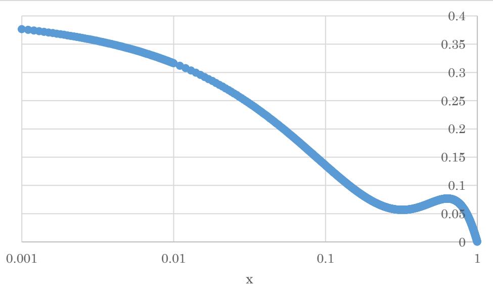<figure data-latex-placement="tbp"> <img src="https://doc.journalspress.com/wq0zzw_226226/author_package/media/ecd89b6257a1d075496d079f5797dbef5d521a4e4828b553788feff1fe622f9b.jpg" style="height:75.0%" /> </figure> Fig. 1 shows temporal sea quarks distribution functions $f _ { \pi ^ { + } } ^ { s e a \bar { d } } ( x )$. Note that $f _ { \pi ^ { + } } ^ { s e a \bar { d } } ( x )$ has two extrema but that important one is extrema of which x value is smaller one. In this case, $x = 0.32$. 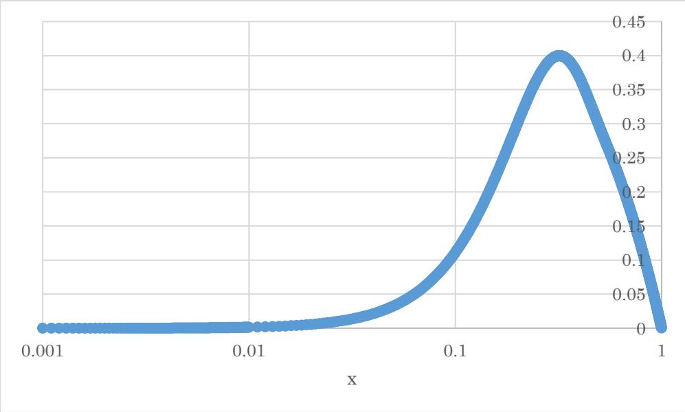Our pion distribution functions of which the $x$ value of the peak point is $x = 0.32$ can be obtained by taking value as $\rho = 5$ in Eq. (2). Fig. 2 shows our u quark distribution functions in the case of $\rho = 5$ , that is one half of our pion distribution functions of which $\rho$ value is $\rho = 5$. <figure data-latex-placement="tbp"> <img src="https://doc.journalspress.com/wq0zzw_226226/author_package/media/6ef2ff120b48ed2d8e866274c0e2f5791c1904038d171753f067fcabf584a466.jpg" style="height:75.0%" /> </figure> Fig. 2 $u ( d )$ quark distribution functions in the case of $\rho = 5$. Note that we adjust the constant of Eq. (2) so that peak value becomes 0.4. Using the adjustment of the constant means removing the requirement of normalization condition that is necessary to obtain the distribution functions of pion as shown in ref. \[8\]. The fact that we need to remove the requirement of normalization condition may also reflect the situation that $u \bar { d }$ system in proton is not exact pion but only close state. However, this adjustment is not so large as shown in the following paragraph. Actual peak value of pion distribution functions in the case of $\rho = 5$ is 0.6217 and peak value of pion distribution functions in the case of $\rho = 3$ is 0.7359 as shown in Fig. 1 of ref. \[8\]. Recalling that u quark distribution functions is obtained by multiplying $\frac { 1 } { 2 }$ to pion distribution functions as shown in ref. \[8\], actual peak value of u quark distribution functions in the case of $\rho = 5$ is 0.31085. 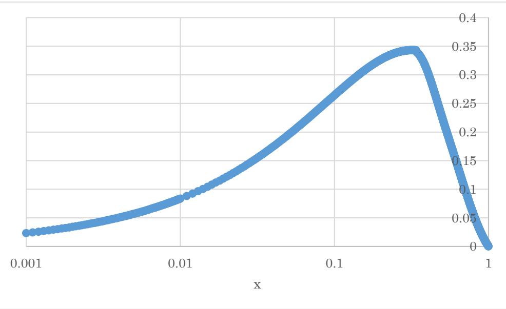Recalling that our definition of valence quark distribution functions, for this case, upper value is 0.4 when range of $x$ is $x \in [ 0 , 0.32 ]$, and upper value corresponds to down slope of u quark distribution functions in the case of $\rho = 5$ when range of x is $x > 0.32$. Then, we obtain the following figure for valence u quark distribution functions come from $\pi ^ { + }$. <figure data-latex-placement="tbp"> <img src="https://doc.journalspress.com/wq0zzw_226226/author_package/media/815bcebd26872288b3480d080306ddc7911c417685097f1ac2b606078452fa96.jpg" style="height:75.0%" /> </figure> Fig. 3 Valence quark distribution functions $f _ { \pi ^ { + } } ^ { v a l u } ( x )$ come from $\pi ^ { + }$. 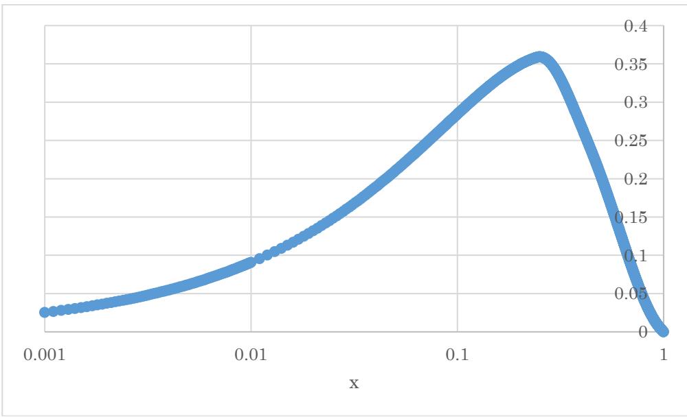Note that the shape of down slope becomes similar to that of valence u quark distribution functions of Atlas experiment results. Comparing the shape of down slope of $f _ { \pi ^ { + } } ^ { v a l u } ( x )$ in Fig.3 to that of u quark distribution functions in the case of $\rho = 5$ in Fig. 2, to obtain our final valence u quark distribution functions $f ^ { v a l u } ( x )$ , the shape of down slope changes only slightly. Thus, over all shape of $f ^ { v a l u } ( x )$ becomes similar to that of Atlas experiment results using subtraction of the temporal sea quarks distribution functions in entire x domain. Therefore, the temporal sea quarks distribution functions must have some meaning which we have not figured out yet. Using the same procedure, we show valence quark distribution functions $f _ { \pi ^ { 0 } } ^ { v a l u } ( x )$ come from $\pi ^ { 0 }$ in Fig. 4. $f _ { \pi ^ { 0 } } ^ { v a l u } ( x )$ has peak at $x = 0.243$. <figure data-latex-placement="tbp"> <img src="https://doc.journalspress.com/wq0zzw_226226/author_package/media/65a46f6f832bc07d0850fb15f00fe241cadf44e6355dc2e03d0b34bb97e043ab.jpg" style="height:75.0%" /> </figure> Fig. 4 Valence quark distribution functions $f _ { \pi ^ { 0 } } ^ { v a l u } ( x )$ come from $\pi ^ { 0 }$. Note that, in our consideration, valence d quark distribution functions $f _ { \pi ^ { 0 } } ^ { v a l d } ( x )$ is same as $f _ { \pi ^ { 0 } } ^ { v a l u } ( x )$. To obtain $f _ { \pi ^ { 0 } } ^ { v a l u } ( x )$ $f _ { \pi ^ { 0 } } ^ { s e a \bar { u } } ( x )$ as shown in Fig. 5. <figure data-latex-placement="tbp"> <img src="https://doc.journalspress.com/wq0zzw_226226/author_package/media/d83f6b6be24333355dfd1b7d2800adef7e2e01b33d799f0494e384589d21936e.jpg" style="height:75.0%" /> </figure> Fig. 5 Temporal sea quarks distribution functions $f _ { \pi ^ { 0 } } ^ { s e a \bar { u } } ( x )$. Note again that, in our consideration, temporal sea quarks distribution functions $f _ { \pi ^ { 0 } } ^ { s e a \bar { d } } ( x )$ is same as that of $f _ { \pi ^ { 0 } } ^ { s e a \bar { u } } ( x )$. To obtain $f _ { \pi ^ { 0 } } ^ { s e a \bar { u } } ( x )$ ,we take $\bar { \gamma }$ as $\bar { \gamma } = 2.8$ to satisfy the condition that $f _ { \pi ^ { 0 } } ^ { s e a \bar { u } } ( x )$ at $x = 0.1$ must be around 0.1. This $\bar { \gamma }$ value gives that $f _ { \pi ^ { 0 } } ^ { s e a \bar { u } } ( x )$ at $x = 0.1$ is 0.1156, and generates that the $x$ value of the first extrema point is $x = 0.243$. Thus, the $x$ value of peak point of $f _ { \pi ^ { 0 } } ^ { v a l u } ( x )$ is $x = 0.243$. We do not show the figure of u quark distribution functions of which the $x$ value of peak point is $x = 0.243$ here, however, corresponding u quark distribution functions is obtained by setting $\rho$ value as $\rho = 7.8$. Recalling that valence u quark distribution functions in proton, $f ^ { v a l u } ( x )$ , are the sum of $f _ { \pi ^ { + } } ^ { v a l u } ( x )$ and $f _ { \pi ^ { 0 } } ^ { v a l u } ( x )$, $f ^ { v a l u } ( x )$ in Fig. 6. <figure data-latex-placement="tbp"> <img src="https://doc.journalspress.com/wq0zzw_226226/author_package/media/a533a608dcda72af50530ea6c311bc599ef024a1d01de9ab54e6b07667b1f796.jpg" style="height:75.0%" /> </figure> Fig. 6 Valence $u$ quark distribution functions $f ^ { v a l u } ( x )$. 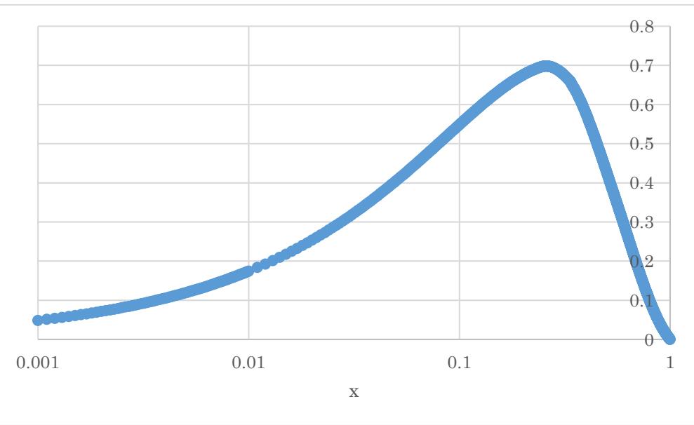Note that the x value of peak point of $f ^ { v a l u } ( x )$ is $x = 0.258$. This $x$ value of peak point is a little bit larger than that of Atlas experiment results (x is around 0.24). For actual sea quarks distribution functions corresponding to $x \bar { u }$ and $x \bar { d }$ denoted as $f ^ { s e a \bar { u } } ( x )$ and $f ^ { s e a \bar { d } } ( x )$ , we simply use the shape of down slope of $f _ { \pi ^ { 0 } } ^ { v a l u } ( x )$ when $x$ is larger than the x value of the first extrema of $f _ { \pi ^ { 0 } } ^ { s e a \bar { u } } ( x ) ( x = 0.243 )$ for $f ^ { s e a \bar { u } } ( x )$, and use the shape of down slope of $f _ { \pi ^ { 0 } } ^ { v a l u } ( x )$ for $f _ { \pi ^ { 0 } } ^ { s e a \bar { d } } ( x )$ and $f _ { \pi ^ { + } } ^ { v a l u } ( x )$ for $f _ { \pi ^ { + } } ^ { s e a \bar { d } } ( x )$ when $x$ is larger than each $x$ value of the first extrema $( x = 0.243 \text{ for } f _ { \pi ^ { 0 } } ^ { s e a \bar { d } } ( x ) \text{ and } x = 0.32 \text{ for } f _ { \pi ^ { + } } ^ { s e a \bar { d } } ( x ) )$. Then, Fig. 7 and Fig. 8 show actual our sea quarks distribution functions $f ^ { s e a \bar { u } } ( x )$ and $f ^ { s e a \bar { d } } ( x )$ , respectively. Note that $f ^ { s e a \bar { d } } ( x )$ is the mean value of $f _ { \pi ^ { 0 } } ^ { s e a \bar { d } } ( x )$ and $f _ { \pi ^ { + } } ^ { s e a \bar { d } } ( x )$. <figure data-latex-placement="tbp"> <img src="https://doc.journalspress.com/wq0zzw_226226/author_package/media/e93b39ea0fea2d3471d26335634906370513904b38b7d91e326419dd0b464151.jpg" style="height:75.0%" /> </figure> Fig. 7 Sea quarks distribution functions $f ^ { s e a \bar { u } } ( x )$. <figure data-latex-placement="tbp"> <img src="https://doc.journalspress.com/wq0zzw_226226/author_package/media/60c0eabca3fee3b4bc3f0704d5e1e36403876b00f53d35cd782cd5dacc8a3a7b.jpg" style="height:75.0%" /> </figure> Fig. 8 Sea quarks distribution functions $f ^ { s e a \bar { d } } ( x )$. Because $\gamma$ in Eq. (13) is represented as $\gamma = \hat { \gamma } / \beta$ , $\gamma = 3.373$ for $\pi ^ { + }$ and $\gamma = 3.675$ for $\pi ^ { 0 }$ . Thus, we can use the form of $\sqrt { | \alpha | }$ as $\sqrt { | \alpha | } = 4 x ^ { 1.55 } ( 1 - x ) ^ { 0.43 }$ for checking the magnitude of the exponential term. For the $\pi ^ { + }$ case, form of exponent becomes $- \frac { \bar { u } } { 4 x ^ { 0.55 } ( 1 - x ) ^ { 1.43 } }$ where $\bar { u } = u / \sqrt { 2 }$ when considering sea quark distribution functions. Because $\rho = 5$ for $\pi ^ { + }$ distribution functions case, that is, 10 times larger than $\rho = 0.5$ corresponding to initial scale (rest frame) distribution functions as shown in ref. \[8\]. That the $\rho$ value is 10 times larger means the $\bar { u }$ value in $\rho$ is 10 times larger. Thus, for sea quarks distribution of $\pi ^ { + }$ we can take $\bar { u }$ as $\bar { u } = 10$ when we take $\bar { u } = 1$ for initial scale. In this case, the exponential almost becomes maximum of about $\exp ( - 10 ) = 4.54 \times 10 ^ { - 5 }$. Actually, even in rest frame (initial scale), proton has sea quarks state. The reason is as follows. The initial scale (rest frame) distribution functions corresponds to the distribution functions before evolution. The distribution functions before evolution must be non-zero, otherwise, sea quarks distribution functions become zero by considering evolution equation, for an example, DGLAP evolution equation \[14\]. Because we consider that sea quarks state is unbound state, the exponential must be sufficiently small even in rest frame because of our definition of unbound state so that the $\bar { u }$ value for initial scale (rest frame) is not 1 but much larger value. For the $\pi ^ { 0 }$ case, $\pi ^ { 0 }$ distribution functions corresponds to the distribution functions in the case of $\rho = 7.8$ , that is, 15.6 times larger. Thus, we can confirm that the magnitude of exponential term, of which exponent is $- \frac { \bar { u } } { 4 x ^ { 0.55 } ( 1 - x ) ^ { 1.43 } }$ ,is negligibly small in entire $x$ domain for both cases. 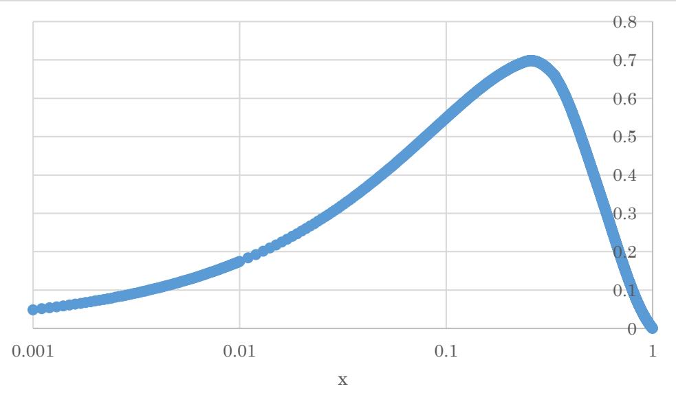# Results We obtain valence u quark distribution functions and valence d quark distribution functions as follows. <figure data-latex-placement="tbp"> <img src="https://doc.journalspress.com/wq0zzw_226226/author_package/media/8f629a2aed5aaa16925f7206f183f8cda4f5b3220d29e1e99b461578b58ceb12.jpg" style="height:75.0%" /> </figure> <figure data-latex-placement="tbp"> <img src="https://doc.journalspress.com/wq0zzw_226226/author_package/media/ba54b0373a63c813eb06124d4bfd017b6918eb766b2121574461012cb5b2bb22.jpg" style="height:75.0%" /> </figure> 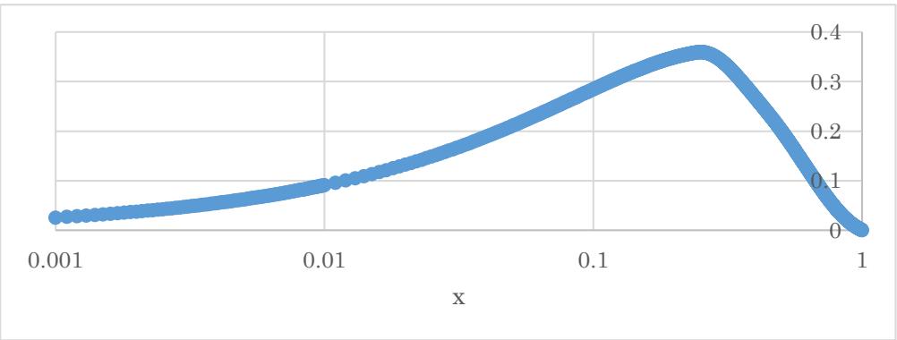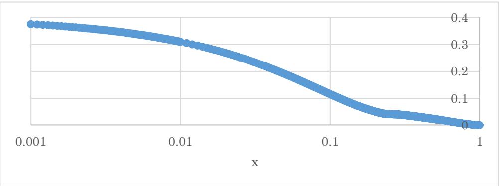Fig. 9 Comparison of valence u distribution functions $f ^ { v a l u } ( x )$ and valence d distribution functions $f ^ { v a l d } ( x )$ upper panel is $f ^ { v a l u } ( x )$ of which the $\mathbf { X }$ value of the peak is $\mathrm { x } = 0 . 2 5 8$ and lower panel is $f ^ { v a l d } ( x )$ of which the $\mathbf { X }$ value of the peak is $\mathrm { x } = 0 . 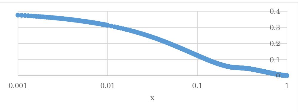2 4 3$ We also obtain sea quarks distribution functions as follows. <figure data-latex-placement="tbp"> <img src="https://doc.journalspress.com/wq0zzw_226226/author_package/media/2f1c779c1f08d6d923da7317c80051ab3973e2b188dff2714661f015aa91b4ca.jpg" style="height:75.0%" /> </figure> <figure data-latex-placement="tbp"> <img src="https://doc.journalspress.com/wq0zzw_226226/author_package/media/fbdfa04e767723a9bb7e9dc096628bae308851e25b31489253f3e57b043faef7.jpg" style="height:75.0%" /> </figure> 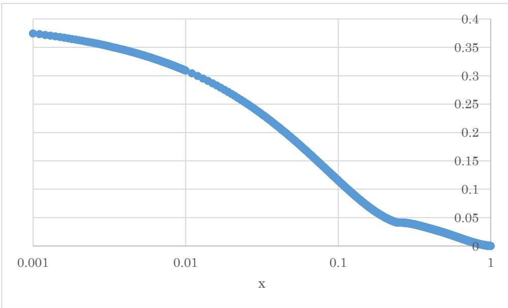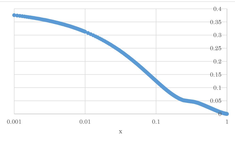Fig. 10 Comparison of sea quarks distribution functions of $f ^ { s e a \bar { d } } ( x )$ and $f ^ { s e a \overline { { u } } } ( x )$ upper panel is $f ^ { s e a \bar { d } } ( x )$ , and lower panel is $f ^ { s e a \bar { u } } ( x )$ <figure data-latex-placement="tbp"> <img src="https://doc.journalspress.com/wq0zzw_226226/author_package/media/05d143c0bba71d2769b64458f56d1a1ed8babf0597dee1b879c5397bc481bf6d.jpg" style="height:75.0%" /> </figure> <figure data-latex-placement="tbp"> <img src="https://doc.journalspress.com/wq0zzw_226226/author_package/media/2da11e34560dfb0b6199b49cdf66ac6089a6aa420dee07083fcefe82a1c44a61.jpg" style="height:75.0%" /> </figure> 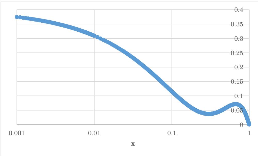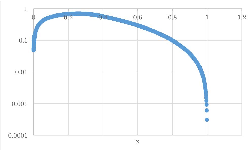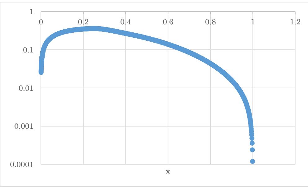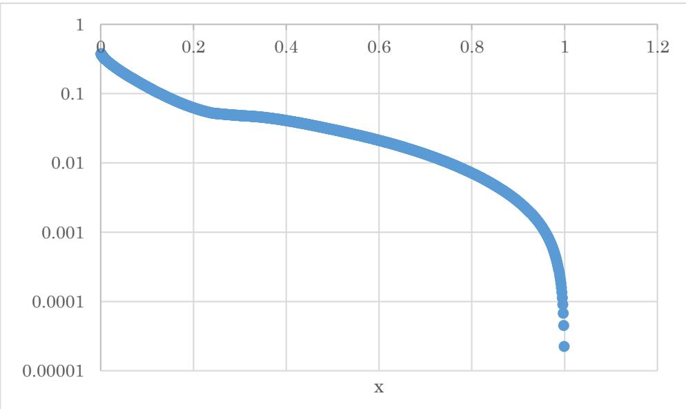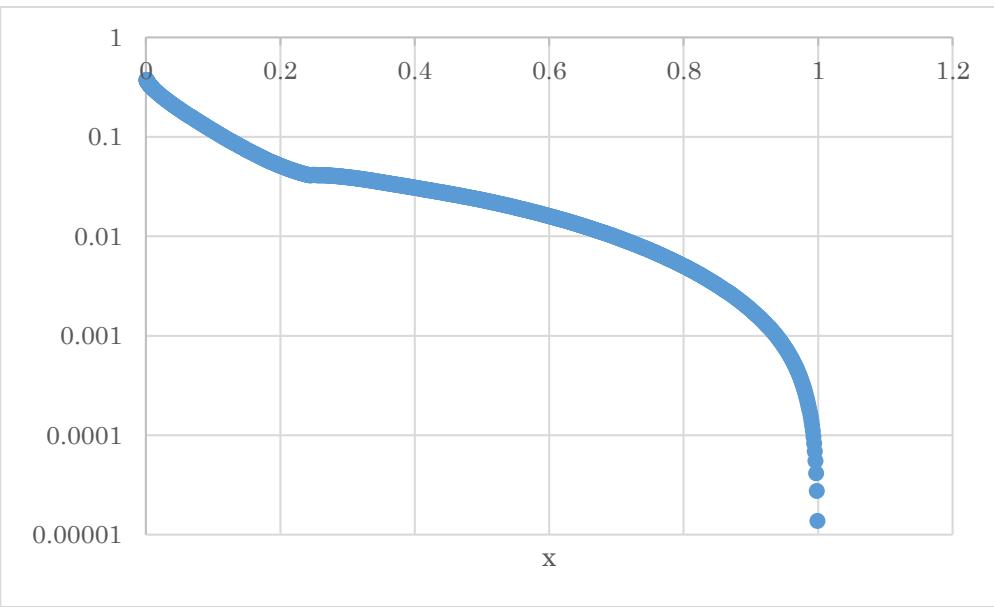Fig. 11 Comparison of valence $\mathbf { u }$ distribution functions $f ^ { v a l } { } ^ { u } ( x )$ and valence d distribution functions $f ^ { v a l \ d } ( x )$ in logarithmic vertical axis (horizontal axis is linear); upper panel is $f ^ { v a l u } ( x )$ , lower panel is $f ^ { v a l \ d } ( x )$ Comparing $f ^ { v a l u } ( x )$ and $f ^ { v a l \ d } ( x )$ ,described in Fig. 9 to Fig.1l, to those of Atlas experiment results, over all shape are similar for both cases and Fig. 11 shows that even value itself is close up to $\mathrm { x } = 0 . 6$ for $f ^ { v a l } { } ^ { u } ( x )$ and up to $\mathrm { x } = 0 . 7$ for $f ^ { v a l \ d } ( x )$ , respectively. <figure data-latex-placement="tbp"> <img src="https://doc.journalspress.com/wq0zzw_226226/author_package/media/d01f4e861be445fe3c32377c33540b0bbb66f61bbd4d9b8c94b038ef41b5a7ef.jpg" style="height:75.0%" /> </figure> <figure data-latex-placement="tbp"> <img src="https://doc.journalspress.com/wq0zzw_226226/author_package/media/93c5f57611300a1f973b48921de2b28d6e098cac45302a1f7d1b452de151feb2.jpg" style="height:75.0%" /> </figure> Fig. 12 Comparison of sea quarks distribution functions of $f ^ { s e a \bar { d } } ( x )$ and $f ^ { s e a \overline { { u } } } ( x )$ in logarithmic vertical axis (horizontal axis is linear); upper panel is $f ^ { s e a \bar { d } } ( x )$ , and lower panel is $f ^ { s e a \ : \overline { { u } } } ( x )$ Comparing $f ^ { s e a } { \bar { d } } ( x )$ to that of Atlas experiment results, over all shape is similar and even value itself is close if we compare it to upper limit of that of Atlas experiment results. Comparing $f ^ { s e a \ : \overline { { u } } } ( x )$ to that of Atlas experiment results, $f ^ { s e a \ : \overline { { u } } } ( x )$ is similar only up to the x value of the first extrema point. In the range of larger than the x value of the first extrema point, Atlas experiment results decrease much faster than $f ^ { s e a \ : \overline { { u } } } ( x )$ However, recalling that we adopt the shape of down slope of valence quark distribution functions corresponding to that in the range larger than the $\mathbf { x }$ value of the first extrema point, we can compare $f ^ { s e a \bar { d } } ( x )$ and $f ^ { s e a \ : \overline { { u } } } ( x )$ to those of Atlas results only up to the $\mathbf { X }$ value of the first extrema. # Conclusion and Discussion We obtain similar behaviors of valence u quark and valence d quark distribution functions to those of Atlas experiment results using the close states described by starting from our charged pion distribution functions with evolution and together with using the ansatz. Actually, this ansatz is technical, however, in reality, systems of $u\bar{u}$ and $d\bar{d}$ are not exact $\pi ^ { + }$ or $\pi ^ { 0 }$ but only close states of these. We think that this ansatz reflects this situation. In addition, this ansatz generates two extrema in each temporal sea quarks states. In addition, x value of the first extrema $f _ { \pi ^ { 0 } } ^ { s e a \bar { d } } ( x ) \sim ( x = 0.243 )$ is very close to x value of peak of valence $d$ quark of Atlas experiment results ($x$ is around 0.2) and for valence u quark distribution functions, x value of the first extrema of $f _ { \pi ^ { 0 } } ^ { s e a \bar { u } } ( x )$ (same as $f _ { \pi ^ { 0 } } ^ { s e a \bar { d } } ( x ) )$ $( x = 0.243 )$ and $x$ value of the first extrema of $f _ { \pi ^ { + } } ^ { s e a \bar { d } } ( x )$ $( x = 0.32 )$ which are same x values of peak points of $f _ { \pi ^ { 0 } } ^ { v a l u } ( x )$ and $f _ { \pi ^ { + } } ^ { v a l u } ( x )$, respectively, and $x$ value of peak point of sum of these, i.e., $f ^ { v a l u } ( x )$ $( x = 0.258 )$ is also very close to valence u quark distribution functions of Atlas experiment results ($x$ is around 0.24). Thus, this ansatz is meaningful. However, as mentioned in Sec. 2, we have not figured out its real meaning yet. Using the shape of down slope of valence u quark or that of $d$ quark distribution functions to obtain sea quarks distribution functions is really technical because we do not know how to estimate this part. Except for this process, we think that our process is reasonable. As a final comment, we consider behavior of $u\bar{d}, u\bar{u}$ and $d\bar{d}$ inside proton as following way. Exact pions decay very quickly so that inside proton pions must be unbound state, however, when x is very small that corresponds to very surface of proton ( r is large), by absorbing gluons, quark and antiquark pair becomes bound state so that confinement potential reappears. Thus, free quarks or antiquarks cannot be observed from proton. Actually, gluon distribution functions becomes decreasing when x is smaller than 0.003. we think this behavior is reflection of above mentioned mechanism. # Appendix A According to standard QCD, sea quarks appears by gluon splitting. In this case, quarks is described as $q\bar{q}$ state that corresponds to exactly coupling constant $g^2 = 0$ case of our definition of [7]. In our case, these are obtained from following two parts. One is from our solution $\chi_3(r)$ ($\sigma_1$ component) [7] which gives to Eq. (1) and Eq. (2). The other one comes from vacuum expectation value $S(r) = \frac{1}{2\pi}Pr\frac{1}{r} (i\sigma_3 \text{ component}) [7]$. To obtain wave function, we use NJR's Word Identity, especially, in our case, as shown in Appendix A in ref. [16]. This gives this part represents $\chi_0(r)$ (Unit component). For distribution amplitude, we use one dimensional Fourier transform that becomes $$ q \int_0^\infty dr J_{\frac{1}{2}}(qr) = q \left( \int_0^u dr J_{\frac{1}{2}}(qr) + \int_u^\infty dr J_{\frac{1}{2}}(qr) \right) $$ Again we consider only First term integral because of considering large $q$ case [7]. Then the first term integral becomes [17] $$ q \int_0^u dr J_{\frac{1}{2}}(qr) = -\frac{1}{2}qu J_{\frac{1}{2}}(qu) + S_{-1, -\frac{1}{2}}(qu) - qu J_{-\frac{1}{2}}(qu) S_{0, \frac{1}{2}}(qu) + 1 $$ where $S_{\mu, \nu}(z)$ denotes Lommel function defined as [18] $$ \begin{aligned} S_{\mu, \nu}(z) &= \frac{ {}_1F_2 \left( 1; \frac{1}{2}(\mu - \nu + 3), \frac{1}{2}(\mu + \nu + 3); \frac{1}{4}z^2 \right) }{ (\mu + 1)^2 - \nu^2 } z^{\mu + 1} \\ &\quad + \frac{2^{\mu-1}\pi^2 \csc(\pi\nu)}{\Gamma\left(\frac{1}{2}(-\mu-\nu+1)\right)\Gamma\left(\frac{1}{2}(-\mu+\nu+1)\right)} \left( J_{-\nu}(z)\sec\left(\frac{1}{2}\pi(\mu+\nu)\right) \right. \\ &\quad \left. - J_{\nu}(z)\sec\left(\frac{1}{2}\pi(\mu-\nu)\right) \right) \end{aligned} $$ Recalling that domain of above $q$ is $[0, \infty]$, $q$ becomes $\frac{x}{1-x}$, $x \in [0, 1]$. In addition, these terms are for distribution amplitude so that this part of distribution functions is obtained by multiplication of $x$. In our case, $\mu=0, \nu=\frac{1}{2}$ explicit description of this term becomes for small $x$ $$ f_{gluon}^{sea2}(x) \approx x \left( 1 + a \sqrt{\frac{1-x}{x}} - b \right) $$ where $a = \frac{1}{\Gamma(\frac{3}{4})\Gamma(\frac{3}{4})} \frac{\pi^2}{2\sqrt{u}}$, $b = 4 + \frac{1}{\Gamma(\frac{3}{4})\Gamma(\frac{3}{4})} \frac{\pi^2}{\sqrt{2}}$. Recalling that, chiral limit case, $m_\pi \to 0$ and that Renner relation such as $\frac{M}{m_\pi} \to \bar{\rho}$ constant, we can consider $\frac{\sqrt{2}}{f_\pi}\bar{\rho}$ as parameter $[C]$. Therefore, we can choose this parameter to cancel out $-x$ term of Eq. (2) obtained by considering $\chi_3(r)$. In addition, we can also use $u$ as parameter. Thus, for small $x$ case, sea quarks distribution functions by gluon splitting up to $x = 0.07$ is described as $$ f_{gluon}^{sea}(x) = 2 \left( 1 - \bar{a}\sqrt{x(1-x)} + bx \right) $$ ($0.001 \le x \le 0.07$) For $0.07 \le x \le 1$, we use the shape of down slope of sum of valence $u$ and valence $d$ quark distribution functions. We choose the shape of down slope to satisfy the condition both curves are smoothly connected at $x=0.07$. 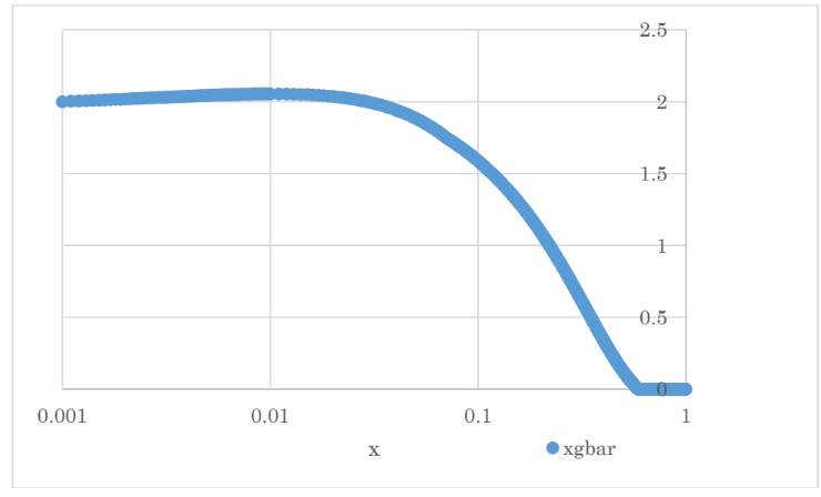This gives following figure for sea quarks distribution functions splitting by gluons (Fig. 13). <figure data-latex-placement="tbp"> <img src="https://doc.journalspress.com/wq0zzw_226226/author_package/media/appendix_fig1.png" style="height:75.0%" /> </figure> Fig. 13 gluon distribution functions of $x\bar{g}$. This is similar to gluon distribution functions of Atlas experiment except range $x=[0.001, 0.003]$. This is understood by considering that distribution functions of $q\bar{q}$ corresponds to that of gluons because we can consider that just after splitting momentum keeps that of just before splitting. From this consideration, we think sea quarks described in Atlas experiment are not generated by gluon splitting. We cannot really clarify the boundary of coupling constant $g^2$ value, however, definitely not exactly zero. This also gives why we use our ansatz besides our argument in Sec. 2.

Generating HTML Viewer...