





IntelliPaper
Abstract
The coupling coordination degree (CCD) is considered to be an important yardstick for guiding practice toward sustainable development. It helps quantitatively investigate the interactions between two or more subsystems within a complex system. However, the existing CCD models have inherent shortcomings. Currently, no consensus has been reached on CCD models. In line with this background, this research proposes a new CCD model from the perspective of the cosine of the high-dimensional spatial angle and develops a novel Excel© tool named Ex-CCD. Taking the coupling coordination analysis between economic-social development, resource consumption, and environmental pollution in China during 2000–2016 as an example, a case demonstration is conducted, and the results show that the model proposed in this research can more accurately describe the coupling coordination state of a system. This new model provides a significant theoretical and practical basis as well as a novel perspective for further coupling coordination research.
Explore Digital Article Text
I. INTRODUCTION
1.1 Research background and significance
According to the Global Sustainable Development Report 2019, The Future is Now: Science for Achieving Sustainable Development, with the continuous increase of population, the intensification of human activities and the economy development, the resources and environment globally are under unprecedented pressure (United Nations, 2019). The shortage of resources and the continuous deterioration of the environment caused by the global population increase and economic-social development seriously threaten the realization of sustainable development goals (SDGs). Moreover, due to the continuous acceleration of urbanization (according to a report released by the United Nations in 2018 (United Nations, 2018), World Urbanization Prospects: The 2018 Revision, the urban population accounted for more than 55% of the world's total population, and this proportion will increase significantly in the future), the contradictions among population, economy, resources, and environment in some areas may become more prominent (Shen et al., 2020). Taking a specific example, Jakarta, the capital of Indonesia, the excessive increase in population and rapid economic-social development in recent years have caused Jakarta to suffer from river pollution, air pollution, insufficient resources, traffic paralysis and other urban problems for a long time (Delinom et al., 2009), even causing Indonesia to decide to move its capital from Jakarta to East Kalimantan Province (Delinom et al., 2009; Nugroho, 2019). Given that resources and the environment continue to provide important guarantees and support for population growth and socioeconomic development, it is imperative to understand the interaction and coordination relationship between the population (including anthropogenic activities), economy, resources, and environment (Li and Yi, 2020; Xiao et al., 2020), which can provide an important guarantee for achieving SDGs (Huan et al., 2021; Li et al., 2021a). The interaction and coordination relationship of the different subsystems is a key issue to realize sustainable development (Li and Yi, 2020). Accordingly, as a measurement, the coupling coordination degree (CCD) was introduced and has become a widely used approach to help understand and analyze the interactions between the different elements in the system in the process of system operation, development and evolution (Shi et al., 2020; Sun et al., 2022). In recent years, CCD research has gradually become a hot spot in the field of sustainable development.
Coupling was originally a physical concept (Etherington et al., 2016). "Coupling" refers to a phenomenon in which multiple systems with multiple connections closely cooperate and rely on each other. "Coupling degree" is a measure of the coupling state (Yang et al., 2017), which refers to the phenomenon that two or more systems or motion forms influence each other through various interactions (Wang et al., 2011). Subsequently, it was widely used in many fields outside of physics. The coupling degree model is only a representation of the strength of interaction between systems and cannot effectively reflect the level of coordinated development. That is, when the development level of both systems is low, a higher degree of coupling can be obtained, but this coupling is not an ideal state. To avoid this deficiency, the coordination degree model is introduced (Fan et al., 2019). The coordination degree is a quantitative indicator to measure the status or level of the development of the elements in a system (Li et al., 2014). This implies that the coupling coordination degree considers not only the interaction degree but also the coordination level of the elements in a system (Li et al., 2012). The interactions of the two subsystems are intricate: they support and hinder each other with time. Coupling coordination refers to the status where subsystems interact and have effects on each other (Liu et al., 2018; Sofowote et al., 2010), and it is proper to analyze the interactions between the subsystems. Coupling coordination reflects how the subsystems interact with each other and how the system evolves from disorder to harmony (Ding et al., 2015). Many studies are dedicated to revealing the complex interactions between different subsystems using the coupling coordination model and its extensions (Zhang and Li, 2020; Zhao et al., 2016; Zhou et al., 2017).
Judging from the existing research status, the understanding of the concepts of coupling degree, coordination degree, and coupling coordination degree are all widely accepted in academia. However, there is still no consensus on the corresponding calculation models. According to the different understandings and cognitions, scholars have made many modifications and improvements based on the original coupling coordination degree model. For example, Feng and his colleagues (Feng et al.,
2021) adopted a modified coupling coordination degree model to investigate the coupling coordination relationship between urbanization and eco-environment. With the help of a modified coupling coordination degree model, Cai and other researchers (Cai et al., 2021) conducted a study on the coupling coordination degree on China's urbanization and agricultural ecological environment at the provincial level. However, due to the inherent shortcomings of the original coupling coordination degree model, none of the modified models overcame the shortcomings.
Therefore, it is imperative to reproduce the calculation model of the coupling coordination degree from a novel perspective. To facilitate the application and promotion of the model, it is necessary to propose a user-friendly calculation tool, which preferably has both a calculation function and a result visualization function, so that the users can understand the calculation results at a glance.
1.2. Literature review and research gap
1.2.1. Summary of the previous literature
In terms of the coupling coordination degree (CCD) modeling approaches proposed in the previous literature, various methods have emerged (Sun et al., 2022; Zhang et al., 2020). These methods are very similar, but there are subtle differences. A detailed summary of the existing CCD evaluation models was conducted in this research, and typical CCD evaluation models were divided into 8 categories (Table 1).
Table 1: Summary of the typical CCD evaluation models presented in previous research
| CCD modeling approaches in the previous literature | The number of elements (n) | Details of elements | References | |
| $CD^{(Coup)} = \sqrt[n]{\frac{\prod_{i=1}^{n} x_i}{\sum_{i=1}^{n} x_i}}$ $CD^{(Coord)} = \sum_{i=1}^{n} w_i \times x_i$ $CCD = \sqrt{CD^{(Coup)} \times CD^{(Coord)}}$ | Model 1 | 2 | Coastal ecology and coastal development level | (Zhang et al., 2019a) |
| 2 | Air environment and tourism | (Geng et al., 2021) | ||
| 2 | Carbon emission and eco-environment | (Chen et al., 2020a) | ||
| 2 | Urbanization rate and rural hollowing index | (Zhang et al., 2019b) | ||
| 3 | Economy, society and environment | (Li and Yi, 2020) | ||
| 2 | Urbanization and ecosystem health | (Li et al., 2021a) | ||
| 4 | Society, economy, environment, means of implementation and cooperation | (Huan et al., 2021) | ||
| 2 | Urbanization and geological hazards | (Zhang and Li, 2020) | ||
| 2 | Economic growth and urban climate change | (Liu et al., 2020a) | ||
| 2 | Supply and demand of ecosystem services | (Xin et al., 2021) | ||
| $CD^{(Coup)} = (\frac{\prod_{i=1}^{n} x_i}{\sum_{i=1}^{n} x_i})$ $\frac{\sum_{i=1}^{n} x_i}{n}$ | Model 2 | 2 | Urbanization and air quality | (Fan et al., 2020) |
| 2 | Forestry management efficiency and forest ecological security | (Chen et al., 2020b) | ||
| $CD^{(Coord)}$ and $CCD^{\star}$ | 2 | Economic development and ecological environment | (Shi et al., 2020) | |
| 2 | Ecological and economic development | (Meng et al., 2021) | ||
| 3 | Food, economy and ecology | (Liu et al., 2020b) | ||
| 3 | Production, living and ecology | (Zhou et al., 2017) | ||
| $CD^{(Coup)} = n \times \sqrt[n]{\frac{\prod_{i=1}^{n} x_i}{\sum_{i=1}^{n} x_i}}$ $CD^{(Coord)}$ and $CCD^{\star}$ | Model 3 | 3 | Land areas of production, living and ecological spaces | (Li et al., 2021b) |
| 3 | Upstream, midstream and downstream of the wind power industry chain | (Dong and Li, 2021) | ||
| 2 | Urbanization and ecosystem service | (Xiao et al., 2020) | ||
| 2 | Urbanization and eco-environment | (Feng et al., 2021) | ||
| $CD^{(Coup)} = \frac{\sqrt[n]{\prod_{i=1}^{n} x_i}}{\frac{\sum_{i=1}^{n} x_i}{n}}$ $CD^{(Coord)}$ and $CCD^{\star}$ | Model 4 | 3 | Water, energy and food systems | (Han et al., 2020) |
| 2 | Urbanization and ecological risk of PAHs | (Han et al., 2021) | ||
| $CD^{(Coup)} = \sqrt[n]{\frac{\prod_{i=1}^{n} x_i}{\sum_{i=1}^{n} x_i}}$ $CD^{(Coord)}$ and $CCD^{\star}$ | Model 5 | 4 | Social development, economic development, resource utilization, and environment system | (Sun et al., 2022) |
| $CD^{(Coup)} = \sqrt[n]{\prod_{i=1}^{n} x_i}$ $CD^{(Coord)}$ and $CCD^{\star}$ | Model 6 | 3 | Economy, society and the environment | (Xu and Hu, 2020) |
| $CD^{(Coup)} = (\frac{\prod_{i=1}^{n} x_i}{\sum_{i=1}^{n} x_i})$ $CD^{(Coord)}$ and $CCD^{\star}$ | Model 7 | 2 | Urbanization and the atmospheric environment | (Liu et al., 2018) |
| $CD^{(Coup)} = \sqrt[n]{\frac{\prod_{i=1}^{n} x_i}{\sum_{i=1}^{n} x_i}}$ $CD^{(Coord)}$ and $CCD^{\star}$ | Model 8 | 2 | Urbanization and the agro-ecological environment | (Cai et al., 2021) |
Model 1 in Table 1 is the original and most commonly adopted CCD evaluation model. According to Model 1, the is calculated by the multiple and the average results of the elements, refers to the sum of the multiple results of the weights (generally referred to as "1/n", where n is the element number) and the element values, and the is the square root of the multiple results of and (a detailed algorithm decomposition of Model 1 is displayed in Section 1.2.2.). With the help of this model, the coupling coordination relationships between the different elements within a certain system have been extensively studied. For example, Geng and his colleagues (Geng et al., 2021) revealed the interactions of China's air environment and tourism. Liu and other researchers (Liu et al., 2020b) studied the relationships among economic growth and urban climate change.
Because of different interpretations, some other CCD evaluation models have been proposed (Table 1 Models 2-8). From the perspective of the development process of the CCD models, Models 2-8 are proposed by researchers on the basis of Model 1. Therefore, Models 2-8 are quite similar to Model 1. It is worth noting that almost all the researchers fully agree with the calculation of and CCD. The controversy among researchers is mainly focused on the calculation method of , which is the core difference among Models 1-8. Another point worth highlighting is that in Models 2-8, the s are all calculated on the results of the multiple results and the average results of the elements. All the above analyses show that, in essence, the differences between Models 1-8 are not large.
1.2.2. Algorithm decomposition of the original CCD model
Algorithm decomposition is the basis of model understanding and a necessary prerequisite for model upgrading. As mentioned above, all the CCD models proposed in the previous literature are similar in essence. Therefore, in this research, a detailed algorithm decomposition was conducted on the initial CCD model, Model 1. Considering the fact that the major controversy among researchers is focused on the calculation of the , we mainly analyze the algorithms of the calculation of . For ease of understanding, we graphically display the algorithm of in Model 1 (Fig. 1).
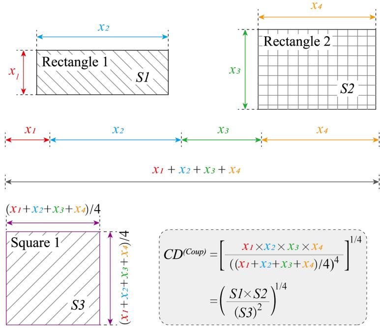 Fig. 1: Graphical algorithm decomposition of the calculation of
in Model 1
Notes: To be more specific, four elements are used to calculate , , CCD. , , , and are the values of these four elements. S1 and S2 represent the areas of Rectangle 1 and Rectangle 2, respectively, and S3 is the area of Square 1. Thus, can be re-expressed as shown in Fig.
In Fig. 1., , and are the widths and heights of Rectangle 1 and Rectangle 2, respectively. A square has been constructed, the width of which is the average of . Then, the equation to calculate can be rewritten as displayed in Fig. 1. From this equation, we find that if a value of the elements refers to 0, the result of will be 0. To be more specific, if there are two systems with 4 elements to calculate, , the values of the elements in the two systems are (10, 7, 9, 0) and (1, 0, 1, 0), respectively, and the results of these two systems will be both 0. Clearly, the results of these two systems are not the same, and the results are quite inaccurate. This phenomenon is a malfunction of the model, named the "failure phenomenon".
represents the overall development level of the different elements within the system (Li et al., 2014; Li et al., 2012). It is generally calculated by the sum of the multiple results of the weights and the element values, and the weights are generally referred to as "1/n", which is the element number (Chen et al., 2020a; Zhang et al., 2019b). CCD refers to the square root of the multiple results between and (Zhang and Li, 2020). and CCD calculation methods have been widely accepted and adopted by almost all researchers.
Moreover, from the graphical algorithm decomposition of in Fig. 1, we can find that the results of have a strong correlation with the results of since the average of the elements ( ) has been used in the calculation process. A case study was conducted to confirm this argument. Virtual data for seven sections each with four elements are displayed in Table 2. A detailed case study for five hundred virtual regions is shown in the Supplemental Material (S1).
Table 2: Virtual data for case study
| Virtual data | $x_1$ | $x_2$ | $x_3$ | $x_4$ |
| Section 1 | 0.1000 | 0.2000 | 0.3000 | 0.4000 |
| Section 2 | 0.2000 | 0.3000 | 0.4000 | 0.5000 |
| Section 3 | 0.3000 | 0.4000 | 0.5000 | 0.6000 |
| Section 4 | 0.4000 | 0.5000 | 0.6000 | 0.7000 |
| Section 5 | 0.5000 | 0.6000 | 0.7000 | 0.8000 |
| Section 6 | 0.6000 | 0.7000 | 0.8000 | 0.9000 |
| Section 7 | 0.7000 | 0.8000 | 0.9000 | 1.0000 |
Calculation results Section 1 Section 2 Section 3 Section 4 Section 5 Section 6 Section 7 0.8853 0.9456 0.9680 0.9788 0.9849 0.9887 0.9913 0.2500 0.3500 0.4500 0.5500 0.6500 0.7500 0.8500 CCD 0.4705 0.5753 0.6600 0.7337 0.8001 0.8611 0.9179
| Calculation results | Section 1 | Section 2 | Section 3 | Section 4 | Section 5 | Section 6 | Section 7 |
| $CD^{(Coup)}$ | 0.8853 | 0.9456 | 0.9680 | 0.9788 | 0.9849 | 0.9887 | 0.9913 |
| $CD^{(Coord)}$ | 0.2500 | 0.3500 | 0.4500 | 0.5500 | 0.6500 | 0.7500 | 0.8500 |
| CCD | 0.4705 | 0.5753 | 0.6600 | 0.7337 | 0.8001 | 0.8611 | 0.9179 |
is a metric used to reveal the degree of coupling of the various elements within the system (Yang et al., 2017), which should be a number independent of the average of , , , and ( ). However, it can be seen in Table 3 that the values of increase significantly as the values of increase (with a correlation coefficient of 0.8603). Such calculation results are caused by the inherent defects of the model, so it is imperative to improve the CCD model from a novel perspective.
1.2.3. Overview of the advantages and shortcomings
In summary, the existing coupling coordination models mainly have the following advantages: 1) The algorithms are very easy to learn and master by new users. In other words, the existing CCD calculation models are very easy to understand, allow new users to quickly begin using them it within a very short period of time. 2) The existing CCD models are very easy for new users to utilize. To be more specific, the calculation processes of the existing CCD calculation methods are relatively simple, and the result can be calculated through the commonly used Excel© software without using any special software or having any programming knowledge.
The main shortcomings can be summarized into the following two aspects: 1) The existing CCD calculation model has an unavoidable failure phenomenon. If one value of the elements refers to o, the result of and CCD will be both o. This causes it to be impossible to accurately calculate the and CCD of the system. 2) should be an index independent of the average value of the elements ( ), revealing the coupling state of the various elements within a system (Chen et al., 2020b). However, using the existing coupling coordination models, the values of increase significantly as the values of increase. This kind of algorithmic confusion between and causes it to be difficult to give specific and effective countermeasures to improve the CCD of the system.
1.3. The main work and innovations of this research
The main work and innovations of this research are mainly reflected in the following aspects: First, this research summarizes the existing CCD algorithms and analyzes the initial CCD algorithm in detail, which has always been lacking in previous CCD studies. Second, this research proposes a novel perspective, the cosine of the high-dimensional spatial angle, to improve the existing CCD evaluation models to eliminate the inherent shortcomings. At the same time, to make the operation of the method proposed in this study more convenient, an Excel© based tool named Ex-CCD was developed. Third, to test the validity of the model proposed in this research, a case study was conducted by taking China's economic and social development, natural resource consumption and environmental pollution coupling and coordination analysis from 2000 to 2016 as an example. The objective of this research is to propose a novel CCD calculation model and provide a user-friendly operating tool.
II. METHOD AND MATERIALS
2.1. A
2.1.1. The initial matrix
We assume that CCD needs to be investigated in h regions. The original data matrix of all the elements of the regions can be expressed as shown in Formula (1).
where is the value of region h's (h=1, 2,..., s) ith (i=1, 2,..., n) element.
2.1.2. Initial data standardization
To eliminate the differences in the magnitudes of the values of different elements and to make the results more comparable, it is necessary to standardize the original data before the calculation process.
{"image_source":{"path":"images/2c5255fdab364f12f5e7fa810e72fc35efbbef7b5166ad954a5a6148030630bb.jpg"},"content":"","chart_caption":[],"chart_footnote":[]}
The min-max normalization method (Peng and Deng, 2020; Bian et al., 2022) was used in this research, as shown in Formula (2). The range of the standardized results is [0, 1].
is the normalized value of region 's ith element.
2.1.3. Weight Determination
The weighting of elements often has a nonnegligible effect on the result (Kurz-Kim, 2010; Uyan, 2014; Gorgij et al., 2017; Sun et al., 2019). Thus, the calculation of element weight is often a key procedure. Generally, weights can be divided into subjective weights and objective weights (Sun et al., 2020; Sun and Yang, 2019). In this study, researchers are allowed to choose the method of weight calculation independently and only need to enter the results of the element weight into the table of the tool developed in this research. If each element is equally important, then the weight setting can be ignored because in the tool, each element is equally important by default, and the value of each weight is 1. In this research, the element weight of element i is denoted as .
2.1.4. The cosine of the high-dimensional spatial angle
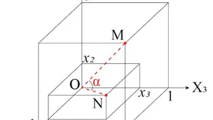
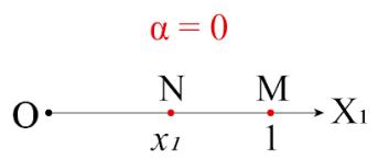
We summarized the general expression form of the cosine of the high-dimensional spatial angle through specific conditions. In other words, by expressing the cosine of the spatial angle when there are one, two, or three elements (Fig. 2.), we obtain the expression of the cosine of the spatial angle when there are multiple elements.
(a) {"image_source":{"path":"images/b998e1f472746eeaeb7b808302e82edd42bc1a055f28da002263a823ae7907a9.jpg"},"content":"","chart_caption":[{"type":"text","content":"(b)"}],"chart_footnote":[]}
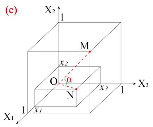
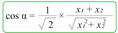 Fig. 2: Illustration of the cosine of the high-dimensional spatial angle
Notes: (n is the number of elements) are the values of the elements for calculating , respectively. Point M is the ideal state point of all of the elements. Point N is the actual state point of all elements. a represents the angle formed by point M, point N, and the origin, point O. It is worth noting that, according to the law of cosines, the minimum and maximum values of cosα are and 1, respectively.
The expressions of the cosine of the spatial angle when there are one, two, or three elements are shown in Fig. 2. We can infer that when there are multiple elements, the expression of the spatial angle cosine is as shown in Formula (3).
The closer the actual state point (N) is to the ideal state point (M), the stronger the interaction between the elements of the system and the greater the degree of coupling. The maximum value of angle is Pi/2, and the cosine function happens to be a monotonically decreasing function in the interval of [o, Pi/2], so the cosine value of is selected to indicate the coupling degree between elements.
2.1.5. The modified coupling coordination degree model
Regarding the CCD model, the main controversy among researchers is the algorithm of the . Therefore, this research mainly improves the algorithm of the through the cosine of the high-dimensional spatial angle, which provides a novel perspective for the calculation of the . The minimum and maximum values of cosα vary with the values of the elements. To eliminate the influence of the number of elements on the result distribution, it is necessary to carry out the standardization operation, as shown in Formula (2). Taking all these aspects into consideration, the calculation methods of the , , and CCD proposed in this study are shown in Formulas (4-6).
where , , and denote the coupling degree, the coordination degree and the coupling coordination degree of region h, respectively.
2.2. Model performance: a case study
To test the performance of the model proposed in this study, we chose to use the model proposed in this study to recalculate the results of the published research and compare the recalculated results with the results of the published research. The case study data comes from (Sun et al., 2022).
In Sun et al. (2022), the researchers established a detailed index system to calculate China's social development, economic development, resource utilization, and environment pollution indices from 2000 to 2016 and calculated the CCDs based on these indices. The values of these indices are shown in Table 4. The data in Table 4 are used as raw data to illustrate the performance of the CCD model proposed in this research.
Table 4: Indices of social development, economic development, resource utilization, and environmental pollution in China during 2000-2016 (Sun et al., 2022)
| Year | Social development | Economic development | Resource utilization | Environment pollution |
| 2000 | 0.11 | 0 | 0.45 | 0.43 |
| 2001 | 0.13 | 0.01 | 0.47 | 0.39 |
| 2002 | 0.16 | 0.03 | 0.57 | 0.47 |
| 2003 | 0.19 | 0.05 | 0.43 | 0.34 |
| 2004 | 0.23 | 0.08 | 0.33 | 0.32 |
| 2005 | 0.27 | 0.11 | 0.45 | 0.53 |
| 2006 | 0.3 | 0.16 | 0.39 | 0.52 |
| 2007 | 0.35 | 0.24 | 0.41 | 0.45 |
| 2008 | 0.4 | 0.34 | 0.47 | 0.62 |
| 2009 | 0.44 | 0.39 | 0.36 | 0.69 |
| 2010 | 0.5 | 0.49 | 0.54 | 0.56 |
| 2011 | 0.57 | 0.64 | 0.31 | 0.61 |
| 2012 | 0.63 | 0.74 | 0.49 | 0.75 |
| 2013 | 0.71 | 0.84 | 0.45 | 0.62 |
| 2014 | 0.78 | 0.93 | 0.45 | 0.64 |
| 2015 | 0.83 | 0.99 | 0.49 | 0.7 |
| 2016 | 0.93 | 1 | 0.63 | 0.8 |
2.3. Tool applicability
Based on the analysis of the existing literature, we found that the number of elements is generally 2-5, and the number of regions to be investigated is usually a few or dozens. To meet the needs of users for the number of elements and regions to the greatest extent, this new Excel-based tool, the Ex-CCD, was designed to conduct coupling coordination analysis of up to 500 regions from up to 15 elements. In addition, the tool developed in this research is capable of handling not only panel data but also time series data. Therefore, this tool can meet the reasonable needs of all groups of users.
2.4. Tool implementation
In this research, "user-centered design (UCD)" is accepted as the basic principle of tool design (Barnum, 2011; Acutis et al., 2022). We coded the Ex-CCD tool in the Excel© environment. UCD is an ISO standard (9241-210: 2019, https://www.iso.org/standard/77520.html), and it is a participatory-based technique. Accordingly, a group of users consisting of Ph.D. candidates, junior and senior researchers were invited to participate in the development of the tool. Designers adjusted the tool according to the feedback of the users. The most frequent feedback from users was the need for a user-friendly tool. In this regard, Excel© is a widely known environment (Berardi, 2002; IZAGIRRE et al., 2007). Excel© allows users with different backgrounds to use the toolkits included in Excel© without mastering the complex algorithms and logics behind these toolkits (Acutis et al., 2022; Jones et al., 2014). These algorithms and logics are more complex than spreadsheet-based solutions. They require coding skills and a deep understanding of the statistical theory behind each test. Moreover, the user interface of the Ex-CCD tool arranges the design of the input and output interfaces very well, and the Ex-CCD tool also includes an operating system with a certain and clear process. A user manual with detailed information can be found in the Supplemental Material (S2). In addition, we also provide a set of video tutorials to introduce the operating steps of the tool.
2.5. Tool effectiveness
To test the accuracy of the Ex-CCD tool, we directly compare the results calculated by using Excel© with those calculated by using the Ex-CCD tool to see if they are consistent. If these two kinds of calculation results are completely consistent, then the tool developed in this research is efficient and accurate. In this study, 500 virtual areas (each area with 4 elements) were used to verify the effectiveness of the Ex-CCD tool. See Supplemental Material (S3) for detailed information on the 500 virtual regions.
III. ILLUSTRATIVE RESULTS AND DISCUSSION
The main contribution of this research is to propose a new CCD calculation model originating from a novel perspective, which is the cosine of the high-dimensional spatial angle. Compared with the existing CCD calculation models, the process of implementing the method proposed in this research using Excel© is very cumbersome, and thus, an Excel-based tool for this model named Ex-CCD has been developed.
The following paragraphs describe the interface, the model performances, and the tool effectiveness analysis.
3.1. Tool interface
As an outcome of the UCD approach, Ex-CCD, the developed Excel-based tool, has a user-friendly interface (Fig. 3.). On the homepage of the tool, we give detailed information about the tool (including operation steps and tutorials).
The tool mainly includes three spreadsheets: the homepage spreadsheet, the input spreadsheet for initial element data and element weights, and the calculation and visualization spreadsheet for the results.
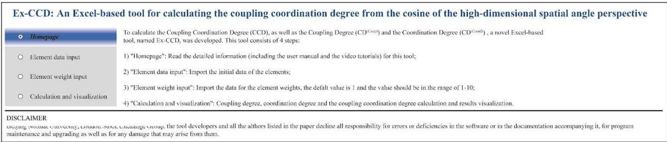 Fig. 3: The Ex-CCD tool introductory screen page
The data input interface is shown in Fig. 4.
| (a) Initial element data used for coupling coordination degree calculation | |||||||||||||||
| Regions\Element data | $a_1$ | $a_2$ | $a_3$ | $a_4$ | $a_5$ | $a_6$ | $a_7$ | $a_8$ | $a_9$ | $a_{10}$ | $a_{11}$ | $a_{12}$ | $a_{13}$ | $a_{14}$ | $a_{15}$ |
| Region 1 | |||||||||||||||
| Region 2 | |||||||||||||||
| Region 3 | |||||||||||||||
| Region 4 | |||||||||||||||
| Region 5 | |||||||||||||||
| $\cdot$ $\cdot$ | |||||||||||||||
| Region 500 | |||||||||||||||
| (b) Element weight | |||||||||||||||
| Element weight | $W_1$ | $W_2$ | $W_3$ | $W_4$ | $W_5$ | $W_6$ | $W_7$ | $W_8$ | $W_9$ | $W_{10}$ | $W_{11}$ | $W_{12}$ | $W_{13}$ | $W_{14}$ | $W_{15}$ |
| Values | 1 | 1 | 1 | 1 | 1 | 1 | 1 | 1 | 1 | 1 | 1 | 1 | 1 | 1 | 1 |
The data input interface mainly contains two parts: one part is about the input of the original data (Fig. 4. (a)), and the other part is about the input of the weights of the different elements (Fig. 4. (b)) (the default value of each weight is 1). Through the standardization process of Formula (2), the data will be distributed in the range of 0-1. To show the calculated results more clearly, we recommend setting the weight value to 1-10 (decimals can be used).
3.1.2. Output
To allow users to obtain a better operating experience, we will display the calculation results and the visualization tables of the same spreadsheet (Fig. 5).
| (a) Standardized data (ah,i) times indicator weight (wi) | (b) Calculation results | |||||||||||||||||
| Values Regions | a1' * w1 | a2' * w2 | a3' * w3 | a4' * w4 | a5' * w5 | a6' * w6 | a7' * w7 | a8' * w8 | a9' * w9 | a10' * w10 | a11' * w11 | a12' * w12 | a13' * w13 | a14' * w14 | a15' * w15 | Coupling degree | Coordination degree | Coupling coordination degree |
| Region 1 | ||||||||||||||||||
| Region 2 | ||||||||||||||||||
| Region 3 | ||||||||||||||||||
| Region 4 | ||||||||||||||||||
| Region 5 | ||||||||||||||||||
| : | ||||||||||||||||||
| : | ||||||||||||||||||
| Region 500 | ||||||||||||||||||
{"image_source":{"path":"images/aead30d536df224083f004e081d54e5f8f0b30ebc0b9521a3401be28ad2bd75e.jpg"},"content":"","chart_caption":[],"chart_footnote":[]} {"image_source":{"path":"images/9bc81d42f06c02da89030a73b3f3401c710442d2547a10197ffca7aec7b1e210.jpg"},"content":"","chart_caption":[{"type":"text","content":"Fig. 5: Calculation results and visualization interface"}],"chart_footnote":[]}
The output page not only displays the final results of the , , and CCD of the investigated areas in the form of a table (Fig. 5. (b)) but also shows the result of multiplying the standardized data and the element weights (Fig. 5. (a)). Moreover, to obtain a more intuitive understanding, the , , and CCD values of the investigated areas are displayed graphically (Fig. 5. (c)). Based on and values the types of coupling coordination states in different regions can be divided (Fig. 5. (d)). If the data for multiple years can be obtained, the evolution path of the CCD can also be displayed.
3.2. Model performance: case study result analysis
The calculation results based on the model proposed in this research and the calculation results of Sun et al. (2022) are shown in Fig. 6. To obtain a more intuitive experience, Fig. 6 also shows the social development index, economic development index, resource utilization index, environment pollution index, and the sum of these indices. Overall, the calculation results of the model proposed in this research and the calculation results of Sun et al. (2022) generally show the similar trends. The results of both models show that the CCD of social development, economic development, resource utilization and environmental pollution in China from 2000 to 2016 generally showed upward trends year by year.
{"image_source":{"path":"images/e9928c0114f1bb9ff34d0762de79861dc49a970732de5505b12e7348da13142b.jpg"},"content":"","chart_caption":[],"chart_footnote":[]}
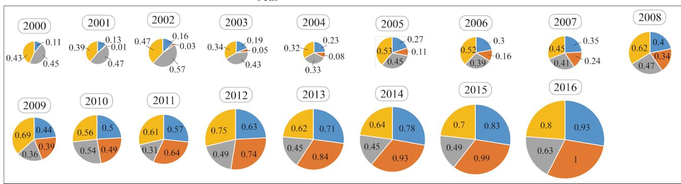 Fig. 6: Comparison of the model proposed in this study with that of Sun et al. (2022)
However, the evaluation results of the two models have slight differences. First, the evaluation model proposed in this research solves the failure problem of the original model (as shown in Fig. 6. Section A). Using the original method, the of the social development, economic development, resource utilization and environmental pollution in China in 2000 could not be accurately calculated, thus they are represented by 0. However, using the model proposed in this research, the of China's social development, economic development, resource utilization and environmental pollution in 2000 can be accurately calculated, which is 0.2415. Second, the evaluation results of the CCD in 2003, 2004, 2009, and 2011 using the two methods have obvious differences, as shown in Fig. 6. Section B, C, D. When calculating , the model proposed in this research starts from the perspective of a multidimensional space and considers the degree of distance from the ideal state of the different coordinates. Therefore, small differences in a single element may cause huge differences in the results. However, the traditional CCD model is only related to the product and average of each element, and the sensitivity is relatively poor. Therefore, it is difficult to accurately measure the CCD of a system. The model proposed in this research is more sensitive and can accurately perceive the of different element combinations. From the sum of the social development, economic development, resource utilization, and environment pollution indices for 2003, 2004, 2009, and 2011, the sum of these indices is significantly lower. However, Sun et al. (2022), which uses the traditional CCD calculation model, did not capture this change well in the calculation results. This also confirms the rationality of the CCD calculation model proposed in this research.
The , , and CCD values calculated by the previous CCD calculation models often have strong correlations. Therefore, in previous studies, and were mostly used as the intermediate process of CCD. According to our investigation, no one has conducted separate analyses of the and in CCD research. However, since the CCD is calculated using and, , the changes in and are very important for understanding the changes in the CCD.
Using the model proposed in this study, we can easily calculate the , , and CCD values and can see the trends of the results intuitively as shown in Fig. 7.
{"image_source":{"path":"images/d494417fd43f5d500e8cd89414349b4fbf3c3ab4ca9e51fa215b1e2e236b875b.jpg"},"content":"","chart_caption":[{"type":"text","content":"Fig. 7: Visualization of the coupling degree, coordination degree and coupling coordination degree"}],"chart_footnote":[]}
Fig. 7 shows the and values derived from social development, economic development, resource consumption and environmental pollution in China from 2000 to 2016. Through Fig. 7, we can see that there is a huge difference between the trend of and the trend of . Fig. 7 shows that showed an upward trend from 2000 to 2007 and then first a declining rising trend from 2007 to 2016. The degree of coordination from 2000 to 2004 showed an upward trend and then a downward trend. The level of coordination in 2004 was the lowest. From 2005 to 2016, the degree of coordination in China showed an upward trend year by year. The CCD also shows a general upward trend year by year. Due to the low values in 2003 and 2004, the CCD in these two years decreased significantly and was at the lowest level of the 2000-2016 period.
Through a two-dimensional Cartesian coordinate system composed of and, , we can understand the changes in the CCD more clearly. If there is only one year of data, then the different types of coupling coordination in the study area can be obtained. To be more specific, it can be determined which areas have high coupling but low coordination or which areas have high coordination but low coupling. In view of the different types of different regions, more effective countermeasures can be given to improve the CCD. If the data are for multiple years, the evolution of the CCD in different regions with the year can be obtained. Fig. 8 shows the evolution path of the coupling coordination of social development, economic development, resource consumption, and environmental pollution in China from 2000 to 2016.
{"image_source":{"path":"images/a69d316c2569c8bf420c8f5fdc31000edb63f3910d52bf12e960c6d6fe1ca923.jpg"},"content":"","chart_caption":[{"type":"text","content":"Fig. 8: Evolution path of CCD analysis"}],"chart_footnote":[]}
It can be seen in Fig. 8 that the evolution trend of the CCD of social development, economic development, resource consumption, and environmental pollution in China from 2000 to 2016 is that from a state where the and are both low, and evolve to a state with a higher and values. The coupling state from 2005 to 2014 is a state of rising volatility, and during this period, the coordination state of the system has been steadily rising.
3.3. Tool effectiveness analysis
The , , and values of the 500 virtual areas directly calculated by Excel© are completely consistent with the results calculated by the Ex-CCD tool. This shows that the Ex-CCD tool developed in this research has very good accuracy. The detailed calculation results are shown in the Supplemental Material (S3). It is worth emphasizing that the data type in this research is time series data. If the data type of the research object belongs to panel data, in order to find out the CCD spatial characteristics, the data calculated by the model proposed in this research needs to be visualized and further analyzed in GIS software.
IV. CONCLUSIONS
The coupling coordination degree (CCD) is a critical yardstick for sustainable development. In recent years, research on the CCD has gradually become a hot spot in the area of sustainable development. CCD can be subdivided into and . Scholars currently have much controversy about the calculation of , and a variety of improved models have been proposed based on the initial calculation model of . However, these models all have deficiencies that cannot be overcome by themselves, such as the "failure phenomenon", the problem of greater correlation between and . These problems greatly limit the future development of research on the CCD.
Based on the classification and summary of the existing CCD models and the algorithm decomposition of the initial CCD model, this research proposes a new calculation method from a brand-new perspective, namely, the cosine of the high-dimensional spatial angle. The CCD is calculated by combining the calculation method proposed in this research and the well-accepted calculation method. To facilitate the application of the CCD model proposed in this research, this research has developed an Excel-based tool for CCD calculation named Ex-CCD. This tool not only has the function of calculating the CCD but is also very easy to utilize and has a complete result visualization function. A case study based on the CCD of social development, economic development, resource utilization and environmental pollution in China from 2000 to 2016 confirmed the rationality of the method proposed in this research and verified the effectiveness of the tools developed in this research.
It is hoped that the model proposed and the tool developed for calculating the coupling coordination degree in this research can be widely adopted and studied in the future.
ACKNOWLEDGMENT
The authors would like to extend special thanks to the editor and the anonymous reviewers for their detailed comments and valuable suggestions. All supporting materials could be found at https://doi.org/10.6084/m9.figshare.23997984.v1.
Conflict of Interest
The authors declare no conflict of interest.
Ethical Approval
Not applicable
Data Availability
The datasets used in this study are openly available at [repository link] and the source code is available on GitHub at [GitHub link].
Funding
This work did not receive any external funding.
References
Cite this article
Related Research


Special Issue
Launch a focused special issue to highlight research, emerging trends, and expert insights in your academic field.
