




IntelliPaper
Abstract
Gross Domestic Product (GDP) of a nation is an important index which reflects health and performance of an economy and its aggregate income. In this paper, annual GDP data of three Asian economies for the time period 1960 – 2022 is used for predictive Autoregressive Integrated Moving Average (ARIMA) modelling. ARIMA is a time series analysis method that can capture temporal tendencies and trends in the data series. We seek to gain insights into the future expected trajectory of economic growth in the selected countries through long-term predictions for the time period 2023 – 2037. Augmented Dick Fuller (ADF) test is used to asses stationarity of the data. In the present empirical study, stationarity at the second order differencing with ARIMA (0, 2, 2) model is identified to predict GDP of China, ARIMA (2, 2, 1) model is identified to predict GDP of Pakistan, and ARIMA (0, 2, 1) model is identified to predict GDP of Bangladesh for the next 15 years. The finding shows that the forecast values of China’s GDP will be $14123.90 per capita in 2023 and $29842.64 per capita in 2037 Pakistan’s GDP will be $1589.066 per capita in 2023 and $2115.446 per capita in 2037, and Bangladesh’s GDP will be $2880.167 per capita in 2023 and $5566.303 per capita in 2037, Our study provides skeletal guidance for governmental bodies and direct investors who rely for business planning and strategizing of the resources on reliable predictions of GDP per capita. Advance knowledge about futuristic GDP level enables administrators, investors and policymakers to make informed economic decisions that may steer economic growth, stability and development in an optimum direction
Explore Digital Article Text
I. INTRODUCTION
Gross Domestic Product (GDP) is a strategic component in the measurement of National Income and Product Accounts. GDP represents the total value of final goods and services. GDP assessment is based on the quantum of consumption and investment by households and businesses in addition to accounting for the governmental expenditure and net exports. GDP is therefore crucial to maintain a stable and progressive economy as it embodies all financial transactions including banking aspects. Planning and decision making for the entire economy is thus conditioned on an accurate information in respect of all the three stakeholders of the economic transactions, namely, households, businesses, and the government, which the indicator GDP can deliver. We thus have an estimated nominal GDP (NGDP) which is used for the purpose of future planning by the finance ministry of the country. The real GDP (RGDP) is obtained after adjusting the estimated NGDP for inflation. The latter is also known as observed GDP in the actual real time. The effective mathematical relationship is represented as, NGDP – inflation rate = RGDP. However, all budget planning and projections utilise the former i.e., NGDP, whereas the common citizen is directly impacted by RGDP. Therefore, fluctuations in the level of covariates of GDP are important in determination of gap between NGDP and RGDP. A country's population is represented by its GDP per capita, or GDP per person. It suggests that an economy's output or income per person can reveal its average productivity or level of living. The terms nominal, real (inflation-adjusted), and purchasing power parity (PPP) can all be used to express GDP per capita. Per-capita GDP considers both the GDP and the population of a nation. Per-capita GDP, when interpreted simply, demonstrates the amount of economic value that can be assigned to each individual citizen. Since value of GDP per person conveniently serves as a measure of affluence, this also translates to a proxy measure of overall national wealth. Per-capita GDP is used by economists to gain understanding of both their own nation's and other nations' domestic productivity. Therefore, it may be crucial to comprehend how each potential covariate affects per-capita GDP growth. In the present paper, we focus on assessment of GDP per capita.
GDP computation is based on the principle of averages which has an upward bias. Therefore, GDP does not capture the income or expenditure or production changes on the regional level. For instance, if a large group of people experience declining income at a time when its complement group in the same population which is smaller in size but experiences upwardly rising incomes, then GDP registers rise. This implies that for the lower income group GDP per capita provides an inflated (and unrepresentative) value. Hence use of GDP at subregional level must be done cautiously. In this paper, we focus on the concept of GDP per capita which gives a more realistic picture of the economic status of a larger entity like nation. GDP represents the current market valuation of the produced goods and services in an economy for the assessment period. This value encompasses spendings and costs on the personal consumption, government purchases, inventories, and the foreign trade balance. Thus, the total capital at stake and covered under GDP envelope of a specific period can be viewed either through (i) production undertaken (ii) income generated or (iii) expenditure accrued for the same period.
The objective of present study is to predict GDP of each of the three selected nations from Asia namely, China, Pakistan, and Bangladesh using times series models. Regression models, time series models, and stochastic approaches are just a few of the numerous forecasting techniques available in statistical literature. The benefit of time series models is that we simply need data for the necessary variable over many time points, which is easily accessible from secondary sources. In contrast to the regression model, where explanatory variables are necessary, we do not require knowledge about other aspects for time series data assessment. Therefore, time series model is the best and easiest method for forecasting which produces results quickly. Time series models for predicting economic variables, such as autoregressive integrated moving average (ARIMA) have grown in favour recently. ARIMA methods are helpful for spotting trends and patterns in time series data that are utilised to provide precise forecasts. Using ARIMA models, the present study seeks to forecast GDP per capita of three selected Asian countries. To create and assess several ARIMA models, we use annual GDP data from 1960 – 2022. Outcome of the present analysis will affect investors who rely on knowledge of future patterns of GDP per capita which impact direction of an economy's growth. These projections would assist in future investment strategies for the business.
Time series ARIMA model for predicting economic patterns based on interdependencies of market forces have been studied by Thomakos and Bhattacharya (2005) forecasted the inflation, industrial output and exchange rates for India, based on univariate ARIMA models and bivariate transfer function and VAR. Ning et al. (2010) who projected GDP for Shaanxi, a province in China, using an ARIMA (1, 2, 1) model over the period 1952 – 2007. Tiwari (2012) emphasizes of the causality between energy consumption (measured in terms of electricity consumption), environmental degradation (measured in terms of CO2 emissions) and economic growth (measured in terms GDP) in India, using Granger approach (in VECM framework), impulse response functions (IRFs) and Variance Decomposition (VDs). ARIMA model based on GDP prediction for Greece has been investigated by Kiriakidis and Kargas (2013). Dritsaki (2015) used an ARIMA (1,1,1) model over the period 1980–2013 to forecast the values of real GDP rate in Greece for 2015, 2016 and 2017. Wabomba et al. (2016) projected Kenya's GDP using an ARIMA (2,2,2) model over the period 1960 – 2012. Yang et al. (2016) projected the annual data of Chinese GDP from 1978 – 2014 using an ARIMA (2, 4, 2) model. Agrawal (2018) studied long-term predictions for GDP in India. Abonazel et al. (2019) used on ARIMA (1,2,1) model over the period 1965 – 2016 to forecast the GDP in Egypt during for the period 2017 to 2026. Eissa (2020) forecasted the GDP per capita for Egypt and Saudi Arabia, respectively, from 2019 – 2030 using the ARIMA (1,1,2) and ARIMA (1,1,1) models based on data from the period 1968 – 2018. Lu (2021) studied both ARIMA and ARIMAX (X is the exogenous variable) approaches to analyze and predict the nonlinear residual of GDP. Ghazo (2021) used ARIMA (3,1,1) and ARIMA (1,1,0) forecast for GDP and Consumer Price Index (CPI) respectively for the Jordanian economy between 2020 and 2022, based on the data from the period 1976 – 2019. Mohamed (2022) used an ARIMA (5,1,2) model for the period between 1960 – 2022 to forecast trajectory of GDP in Somalia for the next fourteen quarters. Polintan et al. (2023) used data from 2018 – 2022 through an ARIMA (1,2,1) model for forecasting GDP in Philippines, for 2022 – 2029 and predicted a steady growth trajectory. Lingale and Riyadh Senan (2023) have used predictive ARIMA (0, 1, 2) model for predicting GDP of India, pertaining to the period 1960 – 2020. Tolulope et al. (2023) used an ARIMA (2,1,2) model for predicting the Nigerian GDP using both in sample and out of sample prediction method, based on data for the period of 1960 – 2020 which correctly indicated a gradual rise in GDP. Dinh (2020) studied to domestic credit growth in Vietnam and China through ARIMA (2,3,1) and ARIMA (2,3,5) models respectively, based on data from the period 1996 – 2017. Lin (2023) analyzed the development of China's financial leasing industry using principal component analysis (PCA) and ARIMA model based on data from the period 2008 – 2021. Zhang et al. (2023) analyzed the problems in China's investment in environmental pollution control, using ARIMA (1,2,1) model based on data from the period 2002–2021. Geo (2023) used on
ARIMA-GARCH model is to predict the law and trend of the stock price change in China, over the period 2017–2019. Zakai (2014) used on ARIMA (1,1,0) model over the period 1953 – 2012 to forecast the GDP in Pakistan. Farooqi (2014) used ARIMA (2, 2, 2) and ARIMA (1, 2, 2) models respectively over the period 1947 – 2013 to forecast the annual imports and exports of Pakistan. Streimikiene et. al. (2018) studied three different time series models such as the AR model with seasonal dummies, ARIMA model, and the Vector Autoregression (VAR) model to forecast the tax revenue of Pakistan for the fiscal year 2016–17 based on the data from the period July 1975–December 2016. The results of this study revealed that among these models the ARIMA model gives better-forecasted values for the total tax revenues of Pakistan. Hussain et al. (2021) used ARIMA (0,1,1) model over the period 1985 – 2015 to forecast the GDP in Pakistan. Amir et al. (2021) forecasted the GDP percentage share on the education of Pakistan from 1971 – 2017 using the ARIMA (2, 1, 1) model. Saleem et al. (2022) forecasted the GDP for Pakistan from 1961 – 2020 by using Box-Jenkins time series methodology. Chawdhary and Hosan (2016) projected Bangladesh's GDP using an ARIMA (2,2,2) model over the period 1970 – 2014. Hussain and Haque (2017) emphasizes the impact of relationship between money supply and per capita GDP growth rate in Bangladesh over the period 1972–2014 with a Vector Error Correlation (VECM) model. Miah et al. (2019) used on ARIMA (1,2,1) model over the period 1960 – 2017 to forecast the GDP in Bangladesh during for the period 2018 – 2030. Ahmad et al. (2019) used on ARIMA (2,1,1) model for forecasting the money value of Bangladesh using the yearly GDP from 1968 – 2017. Voumik and Smrity (2020) forecasted the GDP per capita for Bangladesh from 1972 – 2019 using the ARIMA (0, 2, 1) model. Jahan (2021) used an ARIMA (1,0,1) model for the period between 1961 – 2019 to forecast the economic performance of Bangladesh. Datta (2023) used ARIMA and the autoregressive conditional heteroscedastic (ARCH) methods for the period 1972 – 2020 to investigate the volatility of the growth rates of Bangladesh's real GDP. Ingrisawang (2023) found that the efficiency of forecasting by two combined forecasting model methods (simple-average and Bates-Granger) comprising up to five individual forecasting models based on ranking of the individual forecasting models via correlation coefficients.
In this paper, we estimate and predict the GDP per capita of China, Pakistan, and Bangladesh for next one and half decade by using ARIMA time series model. Section 2 describes model determination methodology used in the present work. Section 3 describes economic stature of the three selected countries from Asia. Section 4 enumerates the models and the model adequacy measures. Section 5 focusses on data description and its analysis. Conclusion and recommendations are summarised in Section 6.
II. METHODOLOGY
Time series models are characterized by the clustering effect or serial correlation in time. In the present paper, we use statistical techniques in time series analysis to estimate and predict GDP of three selected Asian countries through the dynamic ARIMA modelling. ARIMA modelling addresses such issues of dependent errors by introducing time lagged dependent variable and past error terms on the determinant side of the time series model. The model consists of AR, I, and MA segments where AR represents the autoregressive part, I represents Integration indicating the order of differencing in the observed series to achieve stationarity and MA represents the moving average component in the model. ARIMA model fitting is an iterative process that involves four stages; identification, estimation, diagnostic checking and forecasting of time series (Figure 1).
Figure 1: Iterative Modelling Progression for a Stationary Variable in Box-Jenkins Methodology
ARIMA methodology of forecasting is different from most of the other methods because it does not assume any particular pattern or distributional form in the historical data of the series to be forecast. It utilises a general algorithm for identifying a possible model from a general class of models by combining sliding averages in the process under study with spill over from error components in past. The chosen model is then checked against the historical data to see if it can adequately describe the series. Auto-correlation function (ACF) and partial auto-correlation function (PACF) are used to select one or more ARIMA models that seem appropriate during the identification stage. The next stage involves estimating the parameters of a specific Box-Jenkins model (1970) for a given time series. This step verifies the parsimony in terms of the number of model parameters or lack of over-specification by determining whether the selected AR and/or MA parameters have the lowest sum of the squared residuals in addition to the residuals being uncorrelated. A critical and sensitive aspect of an ARIMA model is parsimony. An over-parameterized model cannot predict as efficiently as a sparse model. Model diagnostics and testing is carried out in the third step. Error terms , follow the assumptions for a stationary unvarying process. Drawn from a fixed distribution with a constant mean and variance, the residuals should be white noise (or independent, if their distributions are normal). These prerequisites about the residual distribution are fulfilled by the most adequate Box-Jenkins model. The best model then needs to be decided based on these four paradigms. Thus, testing of the residuals would lead to a better suitable model. A Quantile-Quantile (QQ) plot is a graphical tool which is used to assess the distributional similarity between two plots of datasets. In the context of ARIMA models, a QQ plot is often used to check whether the residuals of the model follow a normal distribution.
III. THE STUDY REGION
The east Asian nation of People's Republic of China (China, henceforth) with a population of more than 1.41 billion is the second most populous nation in the world. It is the third-largest country in the world by total land area, covering around 9596960 square kilometres. China had the fastest economic growth experienced by any nation, going from one of the world's poorest to one of the largest growing economies. With growth rates averaging over the past 30 years, China has emerged as the leading economy with the quickest pace of expansion. China has maintained an improving GDP path owing to its manufacturing sector, export-oriented economy, and workforce sustained on low wages. In 2020, when China's GDP grew by , it was the only significant global economy to do so. However, owing to post COVID-19 economic fallouts in 2022, it experienced one of its worst economic results in decades. After the United States, China is the second-largest economy in the world in terms of nominal GDP, and it is one of the largest economies in the world since 2016, when measured on the basis of purchasing power parity (PPP). World Bank (2022) report credits China's nominal contribution to the global economy in 2022 to about , in PPP terms. World
Bank (2022). South Asian nation Pakistan is also known as the Islamic Republic of Pakistan. With 235.82 million inhabitants, it is the fifth-most populated nation in the world with 881913 square kilometres of land, and as of 2023, it will also have the highest Muslim population in the entire globe with the annual population growth rate of 1.9%. Pakistan is one of the emerging economies, the economy of Pakistan is the 24th largest in the world in the terms of purchasing Power Parity (PPP), and the 41st largest in terms of nominal Gross Domestic Product (NGDP) World Bank (2022). Bangladesh also located in South Asia, is one of the most populous nations in the world with 147516 square kilometres of land. Its population is about 171.18 million, with 1.1% annual growth rate and a high population density of 1265 people per square kilometre. Due to substantial active workforce Bangladesh has a sustained GDP growth since the 1980s. It contributed to robust and consistent GDP growth of 6% per annum in the South Asian region. In terms of nominal Gross Domestic Product (NGDP), Bangladesh is the 34th-largest economy in the world and the 25th-largest economy in terms of PPP as recorded by World Bank (2022).
IV. THE MODEL AND FORECAST
4.1 Autoregressive Model
With the intent to estimate the coefficients p an AR process for univariate model is the one that shows a changing variable regressed on its own lagged values. AR model of order p, or AR(p) is expressed as,
such that all previous study variable values (i < t) will have cumulative impact on the current level accounting for the long-run memory. ACF therefore persists with non-zero realization for a longer time. PACF measures the correlation between an observation k periods ago and the current observation, after controlling for all other observations at the intermediate lags (i.e., all lags\<k). Hence, PACF is useful for determining the maximum order of AR process. PACF(k) = ACF(k) after controlling the effects of . Thus PACF(k) is represented by coefficient of in the regression.
4.2 Moving Average Model
Let be a white noise process, such that t denotes a sequence of independent and identically distributed (iid) random variables with and . Then the qth order MA model which incorporates the dependency between an observation and a residual error is expressed as,
(3) represents impact of past errors on the response variable. Estimated coefficients , , accounting for short term memory help in forecasting.
4.3 Autoregressive Moving Average Model
AR coupled with MA strategy of modelling forms a general class of time series models called Autoregressive Moving Average (ARMA) models intended for use in stationary data series. ARMA (p, q) model is expressed as:
(4) represents a combination of both AR and MA models. In this case therefore, neither ACF nor PACF can solely provide the information on the maximum order of p or q.
4.4 Autoregressive Integrated Moving Average Model
A nonseasonal ARIMA model, where p is the number of autoregressive terms, d is the number of nonseasonal differences needed for stationarity, and q is the number of lagged forecast errors in the prediction model represents a white noise, for p = d = q = 0. In ARIMA there exists no AR part because does not depend on , there is no differencing involved and also there is no MA part since does not depend on . However, if for a general ARIMA model we take a first difference of so that becomes stationary. then d = 1 which implies one time step of differencing.
\begin{array}{I^ccI^cc|} \hline d & 0 & 1 & 2 \ \hline Model & y_t = Y_t & y_t = Yt - Y\{t-1} & y_t = (Yt - Y_{t-1}) - (Y_{t-1} - Y\{t-2}) \ \hline \end{array}
| d | 0 | 1 | 2 |
| Model | $y_t = Y_t$ | $y_t = Y_t - Y_{t-1}$ | $y_t = (Y_t - Y_{t-1}) - (Y_{t-1} - Y_{t-2})$ |
4.5 Model Adequacy Measures
It is necessary to conduct diagnostic checking on the model before using it for forecasting. The residuals that remain after the model has been fitted are deemed sufficient if they are just white noise, and the residuals' ACF and PACF patterns may provide insight into how the model might be improved. Akaike (1973) developed a numerical score that can be used to identify a best model from among several candidate models for a specific data set. Akaike information criterion (AIC) results are helpful when compared to other
AIC scores for the same data set. Smaller AIC score indicates a better empirical fit. Estimated log-likelihood (L) is used to compute AIC as,
such that s is the number of variables in the model plus the intercept term. Schwarz (1978) developed an alternative model comparison score known as Bayesian (Schwarz) information criterion BIC (or SIC) as an asymptotic approximation to transformation of the Bayesian posterior probability of a candidate model expressed as,
Where, L denotes the maximum value of the likelihood function for the model, s is the number of parameters to be estimated by the model, and n is the number of observations in the sample. Although the AIC and SIC values are typically used to select the most appropriate ARIMA model, it should be emphasized that these values are insufficient for determination of the optimum ARIMA model. In the present paper, we first select a model from several possibilities, with the lowest AIC and SIC values, after which the estimated data are subjected to parameter significance tests and residual randomness tests. If the test is successful, then the model is deemed to be the best one; if not, the model corresponding to the second-smallest AIC value and SIC value is selected. Subsequently, the relevant statistical test is re-run. This cycle of trial continues, till the right model is chosen.
4.5 Forecasting
Box-Jenkins method of time series models are applicable only for stationary and invertible time series. Lidiema (2017), Dritsakis and Klazoglou (2019). Future value forecasting can begin once the requirements have been met through procedures like differencing. When the selected ARIMA model confirms to the specifications of a stationary univariate process, then we can use this model for forecasting. Mean Absolute Deviation (MAD), Mean Absolute Percentage Error (MAPE), and Root Mean Square Error (RMSE) statistical measures verify the accuracy of the predictive ARIMA model.
4.6 Forecasting Accuracy
We now present different measures listed to determine accuracy of a predictive model.
(i) Mean Absolute Error
Mean Absolute Error (MAE) calculates the average absolute difference between the predicted values and the actual (observed) values. The absolute differences rather than squared differences make MAE more robust to the outliers. The formula to calculate the MAE is,
Where, n is the number of data points in the dataset, is the actual value of the target variable for data point I and is the predicted value of the target variable for data point i.
(ii) Root Mean Square Error
Root Mean Square Error (RMSE) is a popular accuracy measure in regression analysis and is based on difference between the predicted values of the model and the actual (observed) values in a dataset. Lower RMSE indicate alignment of model's predictions with the actual data. The formula to calculate the RMSE is,
However, due to the squaring of deviations, RMSE give more weight to the outliers and may therefore not be suitable for all types of datasets. Depending on the specific problem and characteristics of the data, other metrics such as Mean Absolute Error (MAE) or R-squared (coefficient of determination) may also be used in conjunction with RMSE to gain a more comprehensive understanding of the model's performance.
(iii) Mean Absolute Percentage Error
Mean Absolute Percentage Error (MAPE) is measuring the percentage difference between the actual (observed) values and the predicted values and it is useful to understand the relative size of the errors compared to the actual values. The formula to calculate MAPE is,
However, it is not well-defined when the actual values are zero or near zero, which can result in non-sensical very large MAPE values.
(iv) Mean Percentage Error
Mean Percentage Error (MPE) instead of taking the absolute percentage difference like in MAPE consider the direction in percentage difference. Thus, accounting for both the positive and the negative magnitude of the errors. The formula to calculate the MAPE is,
Such that the lower values of MPE indicate better forecast accuracy. A value of zero MPE would imply that the forecasted values match the actual values perfectly. However, MPE can have some limitations, such as the potential for the errors to cancel each other out, leading to an artificially low MPE even if the model's performance is not satisfactory.
(v) Mean Absolute Scaled Error
Mean Absolute Scaled Error (MASE) is measuring the performance of a model relative to the performance of a naive or benchmark model. The MASE provides a more interpretable measure of forecast accuracy compared to metrics like Mean Absolute Error (MAE), especially when dealing with time series data and comparing different forecasting models. It provides insights into whether a model is providing meaningful improvements over a basic, naive forecasting approach. The formula to calculate the MASE is,
where n is the length of the series and m is its frequency, i.e., m=1 for yearly data, m=4 for quarterly, m=12 for monthly, etc. MASE measures how well the model performs relative to the naive model's forecast errors taken as benchmark. A value of MASE less than 1 indicates that the model is performing better than the naive model in terms of absolute forecast errors, while a value greater than 1 indicates worse performance than the naive model.
V. DATA AND ANALYSIS
For modelling and forecasting non-seasonal time series data of the annual GDP of the three selected Asian countries of China, Pakistan, and Bangladesh, we have obtained data from the website of World Bank for the period 1960 – 2022. This implies that we have 63 observations of GDP that satisfy the precondition of having over 50 observations for using Box-Jenkins methodology of time series forecasting (Chatfield, 2016).
5.1 Model Identification for GDP
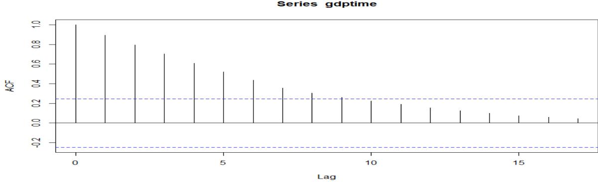
Progression of GDP per capita of China, Pakistan and Bangladesh are graphed respectively in Figure 2 (a), Figure 2(b) and Figure 2 (c). A steady long-term rise is observed during 1960 – 2022. For GDP data beyond 2007 for China, beyond 2018 for Pakistan and beyond 2016 for Bangladesh the rate of upward trend is seen to increase sharply. Such time series may be quickly and easily determined to be unstable because of clearly marked monotonic increasing trend. Figure 3(a), Figure 3 (b) and Figure 3 (c) shows autocorrelation function (ACF) and Figure 4(a), Figure 4(b) and Figure 4(c) shows partial autocorrelation function (PACF) of respectively China, Pakistan and Bangladesh are studied further to understand genesis of data structure. It is evident from the PACF that a single prominence indicates the fictitious primary value of n=1 when it crosses the confidence intervals. Furthermore, at ACF of 10 (height) Figure 3(a), at ACF of 13 (height) Figure 3(b), and at ACF of 9 (height) Figure 3(c), the same issue is observed to occur. According to the ACF plot, the autocorrelations in the observed series is very high, and positive. A slow decay in ACF suggests that there may be changes in both the mean and the variability over time for this series. The arithmetic mean may be moving upward, with rising variability. Variability can be managed by calculating the natural logarithm of the given data, and the mean trend can be eliminated by differencing once or twice as needed to achieve stationarity in the original observed series. An instantaneous nonlinear transformation applied to the optimal forecast of a variable may not produce the transformed variable's ideal forecast (Granger and Newbold, 1976). In particular, using the exponential function to forecast for the original variable when excellent forecasts of the logs are available may not always be the best course of action. Therefore, we further employ the differencing process on the untransformed actual data series.
{"image_source":{"path":"images/c6682dd65f524159d02e0d7a5a859effe4c9aad9e5e7bcb2a9b983d9c37eb426.jpg"},"content":"","chart_caption":[{"type":"text","content":"Figure 2 (a): GDP time series data of China"}],"chart_footnote":[]} {"image_source":{"path":"images/762322f767c6260b1265d3e6e3368ba3b189b9cfd7ca8c8f6e0b9dcc19c5e1f1.jpg"},"content":"","chart_caption":[{"type":"text","content":"Figure 2 (b): GDP time series data of Pakistan"}],"chart_footnote":[]}
{"image_source":{"path":"images/cddc17f909583c402644dde0465d17a20c807e597d23394b8b98c45c928cda20.jpg"},"content":"","chart_caption":[{"type":"text","content":"Figure 2 (c): GDP time series data of Bangladesh"}],"chart_footnote":[]} {"image_source":{"path":"images/0d3e0dc27a15bcf8aa0f442d4e25557ac476ab842de8a53ab913489ba5ec6ec5.jpg"},"content":"","chart_caption":[{"type":"text","content":"Figure 3(a): Autocorrelation function graphs of the GDP of China."}],"chart_footnote":[]}
{"image_source":{"path":"images/212a073863196f6cdd17e7ea9bbb6523a1a77c26f98d47838ad128c541e693c4.jpg"},"content":"","chart_caption":[{"type":"text","content":"Figure 3(b): Autocorrelation function graphs of the GDP of Pakistan."}],"chart_footnote":[]} {"image_source":{"path":"images/42e4b503a0407b787ca00f8cffdcae4bfc7516a4ac83046a1a4cbcd916639dca.jpg"},"content":"","chart_caption":[{"type":"text","content":"Figure 3(c): Autocorrelation function graphs of the GDP of Bangladesh."}],"chart_footnote":[]}
{"image_source":{"path":"images/0e5b67569b20d01a009fec2729864b0eaeba991ce402d63fa5a092fa1e8ca859.jpg"},"content":"","chart_caption":[{"type":"text","content":"Figure 4(a): Partial autocorrelation function graphs of the GDP China."}],"chart_footnote":[]} {"image_source":{"path":"images/443321b60c55ab54927eeac5628e93d55256ad04af8589b551f181f6fb1db236.jpg"},"content":"","chart_caption":[{"type":"text","content":"Figure 4(b): Partial autocorrelation function graphs of the GDP Pakistan."}],"chart_footnote":[]}
{"image_source":{"path":"images/7029fa5834b7f242078ad2fa7538130559bb724c829b2abfc354c223cdc82692.jpg"},"content":"","chart_caption":[{"type":"text","content":"Figure 4 (c): Partial autocorrelation function graphs of the GDP Bangladesh."}],"chart_footnote":[]}
5.2 Estimation and Diagnostics for GDP
Based on GDP time chronological data for the period 1960 - 2022, we consider fifteen tentative ARIMA models (Table 2) and estimate the parameters using R interface. The model with minimum AIC is deemed to fit best and will be referred to as Model I, henceforth.
Table 2: Tentative ARIMA models for GDP of China, Pakistan, and Bangladesh
| Country | China | Pakistan | Bangladesh | |||
| (p,d,q) | Model-I | Model-II | Model-I | Model-II | Model-I | Model-II |
| (2,2,2) | Inf | 970.3199 | 667.2518 | 744.7817 | 673.6429 | 752.0899 |
| (0,2,0) | 909.948 | 1031.373 | 693.5868 | 778.6011 | 688.1801 | 770.0405 |
| (1,2,0) | 889.3717 | 1000.376 | 693.7556 | 779.3334 | 678.3299 | 758.7156 |
| (0,2,1) | 874.2851 | 987.401 | 675.0575 | 755.7337 | 668.5931 | 747.1659 |
| (1,2,1) | 872.3334 | 981.1997 | 673.4915 | 753.9566 | 670.5099 | 749.0751 |
| (2,2,1) | Inf | 974.4929 | 665.5214 | 742.957 | ||
| (1,2,2) | 867.1352 | 971.0277 | 668.4335 | 747.1461 | 671.7747 | 750.2496 |
| (0,2,2) | 865.1353 | 972.1543 | 670.4941 | 749.058 | ||
| (2,2,0) | 681.8224 | 763.2556 | ||||
| (0,2,3) | 867.1352 | |||||
| (1,2,3) | 867.5644 | 972.2159 | ||||
| (3,2,1) | 973.7107 | 667.3552 | 744.8297 | |||
| (3,2,3) | 974.1534 | |||||
| (3,2,0) | 677.0172 | 758.2316 | ||||
| (3,2,2) | 972.1993 | 668.7293 | 746.0844 | |||
If a white noise sequence for residuals is obtained, then Model I is considered suitable for forecast. If not, then the model needs improving. In this paper, the ACF graph Figure 5(a), Figure 5(b), and Figure 5(c) and PACF graph Figure 6(a), Figure 6(b), and Figure 6(c) of residual sequence exhibit white noise process. Hence, ARIMA (0,2,2), ARIMA (2,2,1), and ARIMA (0,2,1), well fits respectively the considered time series GDP data from China, Pakistan, and Bangladesh.
{"image_source":{"path":"images/212c78b048c06f925a2511ca85f582076e5bf0ed9b1740729ee580061ffb6502.jpg"},"content":"","chart_caption":[],"chart_footnote":[]} {"image_source":{"path":"images/dac9eb48667d439dc112ede580ed6d4181f5756943deb9eae4ed966ae6855911.jpg"},"content":"","chart_caption":[{"type":"text","content":"Figure 5 (a): Autocorrelation function graphs of the residual series of China."},{"type":"text","content":"Figure 5 (b): Autocorrelation function graphs of the residual series of Pakistan."}],"chart_footnote":[]}
{"image_source":{"path":"images/4beb2408d82c9a336b4e92952c7ad925204230ebc3e5bef9bc18b45678da50a7.jpg"},"content":"","chart_caption":[{"type":"text","content":"Figure 5 (c): Autocorrelation function graphs of the residual series of Bangladesh."}],"chart_footnote":[]} {"image_source":{"path":"images/c1f7eefecf3e7ae0a2ff7ab5a9257dff6c07ae56c7002d677f045ac3ef5fe12a.jpg"},"content":"","chart_caption":[{"type":"text","content":"Series ts(gdpmodel$residuals)"},{"type":"text","content":"Figure 6 (a): Partial autocorrelation function graphs of the residual series of China."}],"chart_footnote":[]}
{"image_source":{"path":"images/621527e645b7fc1334f8e8a7c5e9411175cbd6a2e163686d7167118deecbf15e.jpg"},"content":"","chart_caption":[{"type":"text","content":"Figure 6 (b): Partial autocorrelation function graphs of the residual series of Pakistan."}],"chart_footnote":[]}
{"image_source":{"path":"images/d2843af74ac0cb2b746aa34ab5b1679f94bf2b20acee295f9277f926ab40c7be.jpg"},"content":"","chart_caption":[{"type":"text","content":"Figure 6 (c): Partial autocorrelation function graphs of the residual series of Bangladesh."}],"chart_footnote":[]}
{"image_source":{"path":"images/79ab6af1458ea41f4cb15a6453294183dbb2e3f01a793a18e4988e37e4147057.jpg"},"content":"","chart_caption":[{"type":"text","content":"Q-Q plot of Residuals"},{"type":"text","content":"Figure 7 (a): Q-Q plot of the residual series of China."}],"chart_footnote":[]}
{"image_source":{"path":"images/c80f55824fa7e520bcdfce6b5089ecf934277ff2db03e46288811b84368c7033.jpg"},"content":"","chart_caption":[{"type":"text","content":"Normal Q-Q Plot"},{"type":"text","content":"Figure 7 (b): Q-Q plot of the residual series of Pakistan."}],"chart_footnote":[]}
{"image_source":{"path":"images/e764d930cb1d279e86487c1dfcc8eeb2a6bb097f98800f8caa25b73d81b2f993.jpg"},"content":"","chart_caption":[{"type":"text","content":"Q-Q plot of Residuals"},{"type":"text","content":"Figure 7 (c): Q-Q plot of the residual series of Bangladesh."}],"chart_footnote":[]}
Figure 7(a), Figure 7(b), and Figure 7(c), illustrates the Normal QQ plot for GDP data as maximum data points fall on or near the straight line. So, it is conceivable that the model residuals are normally distributed for the GDP data of China, Pakistan, and Bangladesh.
Table 3 (a): Estimated Coefficients and Model Adequacy Criterion for China
| Model | I | II | ||||
| Process | $MA_1$ | $MA_2$ | $AR_1$ | $AR_2$ | $MA_1$ | $MA_2$ |
| Coefficients | -1.1479 | 0.7306 | -0.1016 | -0.2427 | -1.0485 | 0.7091 |
| Standard Error | 0.0907 | 0.1336 | 0.2246 | 0.1510 | 0.1962 | 0.1809 |
| AIC | 865.14 | 970.32 | ||||
| BIC | 871.47 | 981.49 | ||||
Table 3 (b): Estimated Coefficients and Model Adequacy Criterion for Pakistan
| Model | I | II | ||||
| Process | $AR_1$ | $AR_2$ | $MA_1$ | $AR_1$ | $AR_2$ | $MA_1$ |
| Coefficients | 0.2820 | -0.4247 | -0.8956 | 0.2826 | -0.4262 | -0.8977 |
| Standard Error | 0.1223 | 0.1273 | 0.0696 | 0.1131 | 0.1098 | 0.0636 |
| AIC | 665.52 | 742.96 | ||||
| BIC | 673.96 | 751.89 | ||||
Table 3 (c): Estimated Coefficients and Model Adequacy Criterion for Bangladesh
| Model | I | II |
| Process | $MA_1$ | $MA_1$ |
| Coefficients | -0.6870 | -0.6881 |
| Standard Error | 0.0846 | 0.0776 |
| AIC | 668.59 | 747.17 |
| BIC | 672.81 | 751.63 |
Table 4: Model Comparison Measures
| Country | Model | RMSE | MAE | MPE | MAPE | MASE |
| China | I | 267.6721 | 133.6117 | 1.847274 | 9.238099 | 0.6440269 |
| II | 247.1423 | 121.6493 | 1.835241 | 8.169301 | 0.3848659 | |
| Pakistan | I | 51.22353 | 34.56317 | 0.6717808 | 7.030863 | 0.8147661 |
| II | 48.24209 | 30.72384 | 0.6064447 | 6.244254 | 0.7433239 | |
| Bangladesh | I | 54.99159 | 30.16532 | 0.01790265 | 9.132468 | 0.6025871 |
| II | 51.79984 | 26.76427 | 0.0175891 | 8.10052 | 0.4038902 |
5.3 Forecasting for GDP
One use of a model is to anticipate the future values of a time series after the model has been discovered, its parameters determined, and its diagnostics examined. Table 6 (a), Table 6 (b) and Table 6 (c) provides the GDP projections for the time window 2023 – 2037. Figure 8 (a), Figure 9 (a), and Figure 10 (a) shows the trend of the actual and forecasted GDP values with their 95% confidence limits for the years 1960 – 2022.
Based on these 63 years, the next 15 years forecasted GDP values for respectively China, Pakistan and Bangladesh is proposed as ARIMA (0,2,2), ARIMA (2,2,1) and ARIMA (0,2,1) based on model I similarly Figure 8 (b), Figure 9 (b), and Figure 10 (b) based on model II. Since the national economy is a complex and dynamic system, and that the outcome is simply a predicted number, therefore in order to prevent the economy from suffering from strong fluctuations, the administrators should maintain
the stability and continuity of microeconomic regulation and control with special attention to the risk of adjustment in economic operation (Wabomba et al. 2016). One should also adjust the corresponding target value in light of the current situation. Thus, to assess robustness of the model-based prediction we next include the first eight predicted values for the years 2023 – 2030 in the original time series data base. The same R program is now re-run for the composite period 1960 – 2030. The ARIMA (2, 2, 2) model for China emerges as the best fit Model II on the new compounded data model on the basis of AIC from among the twelve considered models. Table 3 (a), Table 3 (b), and Table 3 (c) represent the estimated coefficients and model adequacy criterion for both Model I and Model II for respectively China, Pakistan, and Bangladesh under study. Model II estimates have smaller standard errors but AIC and BIC are greater than that of Model I. Model II estimates have smaller RMSE, MAE, MPE, MAPE and MASE (Table 4) for all the three countries, which indicates smaller associated residuals for Model II fit. However, from the viewpoint of sample-based information, of AIC and BIC, Model I of all the three countries are a better representative for the considered actual time series. We predict the next seven annual GDP values for the period 2031 – 2037. 95% confidence interval for Model II are found to be shorter as given in Table 5(a), Table 5(b), and Table 5(c). Thus, retrieving that Model II is more efficient for predictive purpose. However, for all the three selected countries Model I 95% However, for all the three countries model I with 95% confidence band is much wider than that of Model II indicating a less variable model II and therefore better fit.
Table 5 (a): Forecasted values of GDP of China
| Year | Forecasted GDP per capita | 95% Confidence Interval | ||||
| Model -I | Model-II | Model-I | Model-II | |||
| Lower limit | Upper limit | Lower limit | Upper limit | |||
| 2023 | 14123.90 | 13581.78 | 14666.02 | |||
| 2024 | 15246.67 | 14534.42 | 15958.91 | |||
| 2025 | 16369.43 | 15314.76 | 17424.11 | |||
| 2026 | 17492.20 | 15972.79 | 19011.61 | |||
| 2027 | 18614.97 | 16542.36 | 20687.57 | |||
| 2028 | 19737.73 | 17040.86 | 22434.61 | |||
| 2029 | 20860.50 | 17478.11 | 24242.89 | |||
| 2030 | 21983.27 | 17860.46 | 26106.07 | |||
| 2031 | 23106.04 | 23085.49 | 18192.42 | 28019.65 | 22579.23 | 23591.74 |
| 2032 | 24228.80 | 24196.53 | 18477.42 | 29980.19 | 23532.12 | 24860.94 |
| 2033 | 25351.57 | 25311.67 | 18718.21 | 31984.93 | 24382.48 | 26240.85 |
| 2034 | 26474.34 | 26424.24 | 18917.06 | 34031.61 | 25073.64 | 27774.84 |
| 2035 | 27597.10 | 27536.09 | 19075.91 | 36118.30 | 25710.81 | 29361.36 |
| 2036 | 28719.87 | 28648.62 | 19196.42 | 38243.32 | 26313.24 | 30984.01 |
| 2037 | 29842.64 | 29761.27 | 19280.05 | 40405.22 | 26868.00 | 32654.55 |
Table 5 (b): Forecasted values of GDP of Pakistan
| Year | Forecasted GDP per capita | 95% Confidence Interval | ||||
| Model -I | Model-II | Model-I | Model-II | |||
| Lower limit | Upper limit | Lower limit | Upper limit | |||
| 2023 | 1589.066 | 1484.432 | 1693.700 | |||
| 2024 | 1592.068 | 1413.204 | 1770.932 | |||
| 2025 | 1640.259 | 1423.212 | 1857.306 | |||
| 2026 | 1696.676 | 1453.135 | 1857.306 | |||
| 2027 | 1736.221 | 1461.435 | 2011.007 | |||
| 2028 | 1767.513 | 1455.299 | 2079.727 | |||
| 2029 | 1803.644 | 1453.762 | 2153.527 | |||
| 2030 | 1844.645 | 1458.792 | 2230.499 | |||
| 2031 | 1884.964 | 1884.979 | 1462.988 | 2306.941 | 1786.910 | 1983.048 |
| 2032 | 1923.023 | 1923.049 | 1463.461 | 2382.585 | 1755.528 | 2090.569 |
| 2033 | 1960.733 | 1960.763 | 1462.425 | 2459.041 | 1757.727 | 2163.800 |
| 2034 | 1999.306 | 1999.342 | 1461.683 | 2536.929 | 1771.806 | 2226.878 |
| 2035 | 2038.269 | 2038.317 | 1460.794 | 2615.744 | 1781.849 | 2294.785 |
| 2036 | 2076.977 | 2077.035 | 1458.881 | 2695.072 | 1785.841 | 2368.229 |
| 2037 | 2115.446 | 2115.512 | 1455.883 | 2775.009 | 1789.403 | 2441.621 |
Table 5 ©: Forecasted values of GDP of Bangladesh
| Year | Forecasted GDP per capita | 95% Confidence Interval | ||||
| Model -I | Model-II | Model-I | Model-II | |||
| Lower limit | Upper limit | Lower limit | Upper limit | |||
| 2023 | 2880.167 | 2769.724 | 2990.610 | |||
| 2024 | 3072.034 | 2889.757 | 3254.310 | |||
| 2025 | 3263.901 | 3008.029 | 3519.772 | |||
| 2026 | 3455.767 | 3122.115 | 3789.420 | |||
| 2027 | 3647.634 | 3122.115 | 4063.777 | |||
| 2028 | 3839.501 | 3336.101 | 4342.902 | |||
| 2029 | 4031.368 | 3436.032 | 4626.705 | |||
| 2030 | 4223.235 | 3531.423 | 4915.047 | |||
| 2031 | 4415.102 | 4415.100 | 3622.425 | 5207.779 | 4311.358 | 4518.841 |
| 2032 | 4606.969 | 4606.964 | 3709.186 | 5504.751 | 4435.834 | 4778.094 |
| 2033 | 4798.836 | 4798.829 | 3791.848 | 5805.823 | 4558.695 | 5038.962 |
| 2034 | 4990.702 | 4990.693 | 3870.544 | 6110.861 | 4677.656 | 5303.730 |
| 2035 | 5182.569 | 5182.558 | 3945.395 | 6419.743 | 4792.220 | 5572.896 |
| 2036 | 5374.436 | 5374.423 | 4016.517 | 6732.355 | 4902.328 | 5846.518 |
| 2037 | 5566.303 | 5566.287 | 4084.014 | 7048.592 | 5008.062 | 6124.513 |
{"image_source":{"path":"images/58d5725b4fbfdd4da34fc82500f1db858c455555896b92f1eeb85e69ab4cbb88.jpg"},"content":"","chart_caption":[{"type":"text","content":"Forecasts from ARIMA(0,2,2)"},{"type":"text","content":"Figure 8 (a): Time series plot for actual and forecasted GDP values for model I of China."}],"chart_footnote":[]}
{"image_source":{"path":"images/3e7085a56313f5651069f370235a04cf4e39b23cb4c352714542b1ebb8aa90a4.jpg"},"content":"","chart_caption":[{"type":"text","content":"Forecasts from ARIMA(2,2,2)"},{"type":"text","content":"Figure 8 (b): Time series plot for actual and forecasted GDP values for model II of China."}],"chart_footnote":[]}
{"image_source":{"path":"images/46fcd8640dadb530ee01f828c1f3384ff3ac1ee681913d6851d89caa30a79288.jpg"},"content":"","chart_caption":[{"type":"text","content":"Forecasts from ARIMA(2,2,1)"}],"chart_footnote":[]}
{"image_source":{"path":"images/b0c880b4c42e4d11d320e48edbd32420be83471e4719e0a88ce59a431545bdf9.jpg"},"content":"","chart_caption":[{"type":"text","content":"Figure 9 (a): Time series plot for actual and forecasted GDP values for model I of Pakistan."},{"type":"text","content":"Forecasts from ARIMA(2,2,1)"},{"type":"text","content":"Figure 9 (b): Time series plot for actual and forecasted GDP values for model II of Pakistan."}],"chart_footnote":[]}
{"image_source":{"path":"images/b9a28eb5648189826a21ad3e3df0f9aa4fb3f18e8bce23dfb9590772c09e8187.jpg"},"content":"","chart_caption":[{"type":"text","content":"Forecasts from ARIMA(0,2,1)"}],"chart_footnote":[]}
{"image_source":{"path":"images/91b910555e2769ae5a7f1d852a11ccf7b43cd17cdc8577c574d1e192105ba548.jpg"},"content":"","chart_caption":[{"type":"text","content":"Figure 10 (a): Time series plot for actual and forecasted GDP values for model I of Bangladesh."},{"type":"text","content":"Figure 10 (b): Time series plot for actual and forecasted GDP values for model II of Bangladesh."}],"chart_footnote":[]}
VI. CONCLUSION AND RECOMMENDATIONS
Our study discovers that the proposed ARIMA models (Table 2) are useful for future GDP per capita prediction in China, Pakistan, and Bangladesh. For the development and assessment of different ARIMA models, we have used annual data from 1960 – 2022 and found ARIMA (0, 2, 2) model is the most appropriate for GDP of China, ARIMA (2, 2, 1) model is the most appropriate for GDP of Pakistan GDP, and ARIMA (0, 2, 1) model is the most appropriate for Bangladesh GDP. Our findings are in line with earlier research, which discovered that ARIMA models as effective tools of forecasting economic indicators like GDP. Our present study makes a practical contribution by providing in-depth explanations of how ARIMA models might be used to predict per-capita GDP. The best fitted ARIMA model has been used to obtain forecast values for next one and half decade. The finding shows that the forecast values of China's GDP will be $14123.90 per capita in 2023 and $29842.64 per capita in 2037. Forecast values of Pakistan's GDP will be $1589.066 per capita in 2023 and $2115.446 per capita in 2037 and forecast values of Bangladesh's GDP will be $2880.167 per capita in 2023 and $5566.303 per capita in 2037. The results show that all the three economies are in a growing phase. It is therefore suggested to the policy maker to diversify investment on areas of infrastructure development, research, and development, and to facilitate establishment of more startups with focus on green investment and sustainability.
Model II for each considered economy reinforces that short-term prediction of GDP is more precise Table 5(a), Table 5(b), and Table 5(c). Model based prediction enable planners to address specific economic challenges such as resource allocation. A robust GDP prediction could guide the government about the expected revenue generation, and expenditure optimization. Business and governments could plan investment, inventory management and volume of production Statistical prediction thus empowers a decision maker with scope for evidence informed decision-making. However, one must be always aware that any model is sustainable as long as the background conditions such as other influencing market forces remain at the current level. Since GDP addresses only the recorded income on an average, therefore it is not an adequate measure on measuring sustainable development of people in the economy, which can be addressed through Human Development Index which is currently focus of our future research.
ACKNOWLEDGEMENTS
The authors would like to thank World Bank and Ministry of finance, government of China, Pakistan, and Bangladesh for making data available online. The first author is grateful to IoE, University of Delhi for R & D grant.
Declarations
Ethical Approval
Not Applicable
Conflict of Interest
The authors declare no competing interests.
Conflict of Interest
The authors declare no conflict of interest.
Ethical Approval
Not applicable
Data Availability
The datasets used in this study are openly available at [repository link] and the source code is available on GitHub at [GitHub link].
Funding
This work did not receive any external funding.
References
Cite this article
Related Research



Special Issue
Launch a focused special issue to highlight research, emerging trends, and expert insights in your academic field.
