

IntelliPaper
Abstract
This paper deal an AC Transmission system power flow controlled by injecting a compensating voltage in series with the line and injecting reactive power in shunt with the bus. Static Synchronous Series Compensator (SSSC) is considered as a series compensator and Static Synchronous Compensator (STATCOM) is considered as a shunt compensator, while Unified Power Flow Controller (UPFC) is considered as a series-shunt compensator. This paper covers, in depth, the simulation and modeling methods required for study of the steAady-state operation of electrical power systems with these flexible AC Transmission Systems (FACTS) controllers. MATLAB?? codes are used for the implementation of the three devices in the Newton-Raphson algorithm. Power flow control ranges are evaluated for IRAQI (400kV) National Super Grid System (INSGS). Results are studies and reported are presented to compare the effectiveness of the STATCOM, SSSC and UPFC.
Explore Digital Article Text
I. INTRODUCTION
Result for the high demand for electrical power and the higher industrial loads. This provides the need for electricity generating plants and building new transmission lines, a solution that involves long construction times and is costly to implement. So other ways of high the power transfers of existing transmission facilities while in same time maintaining acceptable levels of stability should be considered and network reliability.
FACTS-devices can be used to improve the stability, increase the transmission capacity and ensure better power quality or dynamic behavior in modern power systems. Their main capabilities are voltage control, reactive power compensation and power flow control . FACTS-devices provide fast control in comparison to conventional devices the same phase shifting transformers with mechanical on-load tap changers or switched compensation.
The first of FACTS-devices was mechanically controlled inductors and capacitors. The second of FACTS devices used the thyristor valve control instead of the mechanical switches. The second of FACTS devices gave improvement the enhancement in concept to mitigate the disturbances and in the speed. The third of FACTS devices uses the concept of voltage source converter-based devices. These devices deliver multi-dimensional control the parameters of the power system [7], [8].
II. POWER FLOW CONTROL
The power transmission line can represent by a two-bus system "k" and "m" in the ordinary form [6]. The active power transmitted between bus nodes k and m is given by:
P = \frac {V _ {m} * V _ {k}}{X} \sin (\delta_ {k} - \delta_ {m}Where and are the voltages at the nodes, the angle between the voltages and the line impedance. The power flow can be controlled by altering the voltages at a node, the angle between the end voltages and the impedance between the nodes. The reactive power is given by:
III. NEWTON-RAPHSON POWER FLOW
In large-scale power flow studies, the Newton-Raphson [8] has provided successful and strong characteristics. The expressed power flow Newton-Raphson algorithm by the following relationship:
Where and are bus reactive and active power mismatches, while V and are bus magnitude and angle, respectively.
IV. MODELING OF POWER SYSTEMS WITH STATCOM
The represent of STATCOM by a synchronous voltage source with minimum and maximum of the voltage magnitude limits . The voltage source stands for the fundamental Fourier Series component of the switched voltage waveform at the ac converter terminals of the STATCOM. The bus of the STATCOM is connected is represented as a PV bus, which may be changed to a PQ bus in the case of limits being violated. In this case, the absorbed or generated reactive power would reach the maximum limit. The STATCOM is used to find the mathematical model of the controller for incorporation in power flow algorithms . The STATCOM equivalent circuit shown in Figure 1.
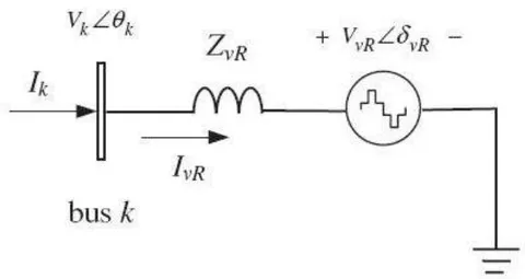
The power flow equations are derived below for the STATCOM
Figure1show a based on the shunt connection, the following equation can be written:
The following reactive and active power equations are obtained for the bus k and converter, respectively, after performing some complex operations:
The linearized STATCOM model is given below, by using these power equations, where the phase angle and the voltage magnitude are taken to be the state variables [4]:
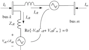
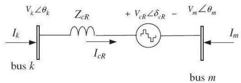
The circuit model of the SSSC connected to link k–m is shown in Figure. The objective of the SSSC is to control the active power to a target value . The SSSC is modeled as a voltage source (VCR) with the angle and adjustable magnitude in series with an impedance. The real part of this impedance represents the coupling transformer and the ohmic losses of the power electronic devices. The imaginary part represents the leakage reactance of the coupling transformer. The admittance (Ys) represents the combined admittances of the SSSC and the line to which it is connected [9] shown in Figure 2. The presence of two new variables ( and ) to the power flow problem. Thus, two new equations are needed for power flow solution. One of these equations is found by ( ) equating to its target value, and the other one is found using the fact that the power consumed by the source ( ) is equal to zero. The power flow equations for all buses of the power system with SSSC in place are the same as those of the system without the SSSC, excluding buses k and m [8].
The SSSC voltage source is:
The phase angle( ) and magnitude ( ) of the voltage source representing the series converter are controlled between limits ( ) and ( ) respectively. From the equivalent circuit shown in Figure 2 and Equations (11), the active and reactive power equations at bus k are:
\begin{array}{l} P _ {k} = V _ {k} ^ {2} G _ {k k} + V _ {k} V _ {m} \left[ G _ {k m} \cos \left(\theta_ {k} - \theta_ {m}\right) \right. \\\quad \left. + B _ {k m} \sin \left(\theta_ {k} - \theta_ {m}\right) \right] + V _ {k} V _ {c R} \left[ G _ {k m} \cos \left(\theta_ {k} - \delta_ {c R}\right) \right. \\\quad \left. + B _ {k m} \sin \left(\theta_ {k} - \delta_ {c R}\right) \right] \\Q _ {k} = - V _ {k} ^ {2} B _ {k k} + V _ {k} V _ {m} \left[ G _ {k m} \sin \left(\theta_ {k} - \theta_ {m}\right) \right. \\\quad \left. - B _ {k m} \cos \left(\theta_ {k} - \theta_ {m}\right) \right] + V _ {k} V _ {c R} \left[ G _ {k m} \sin \left(\theta_ {k} - \delta_ {c R}\right) \right. \\\quad \left. - B _ {k m} \cos \left(\theta_ {k} - \delta_ {c R}\right) \right] \end{array} \tag {1}\tag{12}(13) And for series converter are:
(15)
The system of equations is as follows:
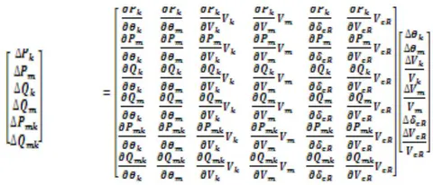
(16)
V. MODELING OF POWER SYSTEMS WITH UPFC
An equivalent circuit of UPFC consisting of two coordinated synchronous voltage sources should represent the UPFC adequately. An equivalent circuit of UPFC shown in Figure 3. The synchronous voltage sources represent the fundamental Fourier series component of the switched voltage waveforms at the AC converter terminals of the UPFC [7].
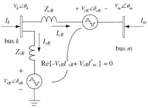
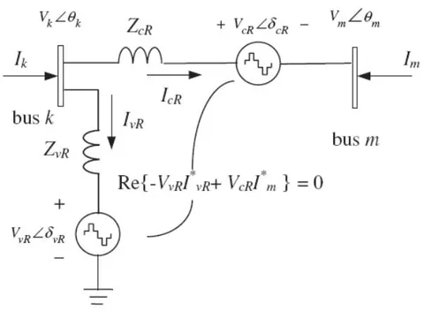
The UPFC voltage sources are:
Where and are the controllable phase angle and magnitude () of the voltage source representing the shunt converter. The phase angle and magnitude of the voltage source representing the series converter are controlled between limits angle and respectively. The phase angle of the series injected voltage determines the mode of power flow control. If is in phase with the nodal voltage angle , the UPFC regulates the terminal voltage. If is in quadrature with respect to , it controls active power flow, acting as a phase shifter. If is in quadrature with the line current angle then it controls active power flow, acting as a variable series compensator [3]. At any other value of/, the UPFC operates as a combination of the voltage regulator, variable series compensator, and phase shifter. The magnitude of the series-injected voltage determines the power flow be controlled. Based on Equations (17) and (18) and the equivalent circuit shown in Figure 3, the reactive and active power equations are at bus k [4]:
\begin{array}{r l} P _ {k} = & V _ {k} ^ {2} G _ {k k} + V _ {k} V _ {m} [ G _ {k m} \cos (\theta_ {k} - \theta_ {m}) \\& + B _ {k m} \sin (\theta_ {k} - \theta_ {m}) ] + V _ {k} V _ {c R} [ G _ {k m} \cos (\theta_ {k} - \delta_ {c R}) \\& + B _ {k m} \sin (\theta_ {k} - \delta_ {c R}) ] + V _ {k} V _ {v R} [ G _ {v R} \cos (\theta_ {k} - \delta_ {v R}) \\& + B _ {v R} \sin (\theta_ {k} - \delta_ {v R}) ] \\Q _ {k} = & - V _ {k} ^ {2} B _ {k k} + V _ {k} V _ {m} [ G _ {k m} \sin (\theta_ {k} - \theta_ {m}) \\& - B _ {k m} \cos (\theta_ {k} - \theta_ {m}) ] + V _ {k} V _ {c R} [ G _ {k m} \sin (\theta_ {k} - \delta_ {c R}) \\& - B _ {k m} \cos (\theta_ {k} - \delta_ {c R}) ] + V _ {k} V _ {v R} [ G _ {v R} \sin (\theta_ {k} - \delta_ {v R}) \\& - B _ {v R} \cos (\theta_ {k} - \delta_ {v R}) ] \end{array} \tag {1}\tag{19}At bus m:
(20)
Series converter:
Shunt converter:
The equations of UPFC power, in linearized form, are combined with those of the AC network. For the case when the UPFC controls the following parameters:
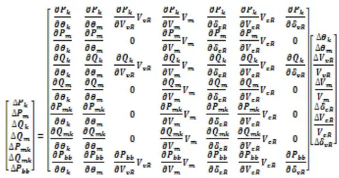
(27)
VI. SIMULATION RESULTS
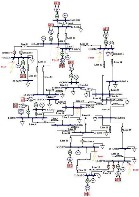
IRAQI (400kV) National Super Grid System (INSGS) network is tested with or without UPFC, SSSC, and STATCOM, to check real Power Losses and reactive Power Losses in the system. In the table (1) we will note the results with and without adding UPFC in all the lines of the system. In the table (2) we will note the results with and without adding SSSC in all the lines of the system. In the table (3) we will note the results with and without adding STATCOM in all the bus of the system.
| Line No. | Location of SSSC | Total Generation System [p.u] | Total Load System [p.u] | Total Real Losses System p.u | Total Reactive Losses System p.u | |||
| Bus number | Real | Reactive | Real | Reactive | ||||
| System with SSSC | 1 | 1-8 | 58.481 | 21.9332 | 58 | 28.5138 | 0.48095 | -6.5806 |
| 2 | 1-14 | 58.4567 | 22.0626 | 58 | 28.5138 | 0.45978 | -6.4512 | |
| 3 | 1-22 | 58.4671 | 21.0039 | 58 | 28.5138 | 0.41709 | -65099 | |
| 4 | 1-22 | 58.4671 | 21.0039 | 58 | 28.5138 | 0.46709 | -6.5099 | |
| 5 | 2-12 | 58.451 | 22.00711 | 58 | 28.5138 | 0.45999 | -6.4427 | |
| 6 | 2-12 | 58.451 | 22.00711 | 58 | 28.5138 | 0.45999 | -6.4427 | |
| 7 | 3-4 | 58.4808 | 21.9181 | 58 | 28.5138 | 0.4808 | -6.5956 | |
| 8 | 3-7 | 58.4509 | 22.3507 | 58 | 28.5138 | 0.4509 | -6.1631 | |
| 9 | 3-12 | 58.4796 | 22.4408 | 58 | 28.5138 | 0.47987 | -6.043 | |
| 10 | 3-12 | 58.4796 | 22.4408 | 58 | 28.5138 | 0.47987 | -6.043 | |
| 11 | 3-13 | 58.4209 | 22.425 | 58 | 28.5138 | 0.42092 | -6.0213 | |
| 12 | 4-5 | 58.4634 | 22.1403 | 58 | 28.5138 | 0.46335 | -6.3735 | |
| 13 | 5-15 | 58.4549 | 22.5858 | 58 | 28.5138 | 0.42493 | -5.928 | |
| 14 | 5-19 | 58.4777 | 21.9261 | 58 | 28.5138 | 0.4777 | -6.5877 | |
| 15 | 6-16 | 58.4777 | 21.9261 | 58 | 28.5138 | 0.4777 | -6.5877 | |
| 16 | 6-16 | 58.471 | 21.5852 | 58 | 28.5138 | 0.47095 | -5.9286 | |
| 17 | 7-13 | 58.4775 | 22.3015 | 58 | 28.5138 | 0.47746 | -6.2124 | |
| 18 | 7-21 | 58.458 | 22.0481 | 58 | 28.5138 | 0.45795 | -6.4657 | |
| 19 | 8-14 | 58.4178 | 22.3877 | 58 | 28.5138 | 0.44777 | -6.1261 | |
| 20 | 9-11 | 58.4301 | 22.3909 | 58 | 28.5138 | 0.43012 | -6.1229 | |
| 21 | 9-20 | 58.4427 | 22.3875 | 58 | 28.5138 | 0.44265 | -6.1263 | |
| 22 | 9-23 | 58.4806 | 22.0792 | 58 | 28.5138 | 0.48063 | -6.4346 | |
| 23 | 10-11 | 58.4806 | 22.0792 | 58 | 28.5138 | 0.48063 | -6.4346 | |
| 24 | 10-11 | 58.4651 | 22.2671 | 58 | 28.5138 | 0.46509 | -6.2467 | |
| 25 | 10-24 | 58.479 | 22.0344 | 58 | 28.5138 | 0.47897 | -6.4794 | |
| 26 | 13-16 | 58.479 | 22.0344 | 58 | 28.5138 | 0.47897 | -6.4794 | |
| 27 | 13-18 | 58.4808 | 22.0024 | 58 | 28.5138 | 0.48077 | -6.5115 | |
| 28 | 14-17 | 58.4751 | 22.0284 | 58 | 28.5138 | 0.47511 | -6.4854 | |
| 29 | 14-17 | 58.4751 | 22.0284 | 58 | 28.5138 | 0.47511 | -6.854 | |
| 30 | 14-18 | 58.4747 | 22.0448 | 58 | 28.5138 | 0.4747 | -6.4691 | |
| 31 | 14-23 | 58.4774 | 22.3482 | 58 | 28.5138 | 0.47739 | -6.1656 | |
| 32 | 15-16 | 58.4781 | 21.9391 | 58 | 28.5138 | 0.47808 | -6.5747 | |
| 33 | 15-17 | 58.4803 | 21.9774 | 58 | 28.5138 | 0.48025 | -6.5364 | |
| 34 | 15-17 | 58.4803 | 21.9774 | 58 | 28.5138 | 0.48025 | -6.5364 | |
| 35 | 15-19 | 58.4797 | 22.0342 | 58 | 28.5138 | 0.47964 | -6.4796 | |
| 36 | 17-20 | 58.4409 | 21.8813 | 58 | 28.5138 | 0.44088 | -6.6325 | |
| 37 | 20-24 | 58.4757 | 22.5755 | 58 | 28.5138 | 0.47568 | -5.9383 | |
| 38 | 22-23 | 58.4686 | 22.2206 | 58 | 28.5138 | 0.46859 | -6.2932 | |
| 39 | 22-23 | 58.4686 | 22.2206 | 58 | 28.5138 | 0.4685 | -6.2932 | |
| without SSSCLine No.Location Of UPFC | 58.481Total Generation System [p.u] | 21.9154 | 58 | 28.5138 | 0.48095 | -6.5984 | ||
| Bus number | Real | Reactive | Real | Reactive | ||||
| System with UPFC | 1 | 1-8 | 58.481 | 21.9332 | 58 | 28.5138 | 0.48095 | -6.5806 |
| 2 | 1-14 | 58.4577 | 22.0453 | 58 | 28.5138 | 0.47774 | -6.4685 | |
| 3 | 1-22 | 58.4657 | 21.9898 | 58 | 28.5138 | 0.45166 | -6.524 | |
| 4 | 1-22 | 58.4657 | 21.9898 | 58 | 28.5138 | 0.46566 | -6.463 | |
| 5 | 2-12 | 58.4579 | 22.0508 | 58 | 28.5138 | 0.49793 | -6.463 | |
| 6 | 2-12 | 58.4579 | 22.0508 | 58 | 28.5138 | 0.45793 | -6.463 | |
| 7 | 3-4 | 58.4808 | 21.9181 | 58 | 28.5138 | 0.4808 | -6.5957 | |
| 8 | 3-7 | 58.4493 | 22.3226 | 58 | 28.5138 | 0.49432 | -6.1912 | |
| 9 | 3-12 | 58.4797 | 22.4697 | 58 | 28.5138 | 0.47965 | -6.0441 | |
| 10 | 3-12 | 58.4797 | 22.4697 | 58 | 28.5138 | 0.47965 | -6.0441 | |
| 11 | 3-13 | 58.4133 | 22.429 | 58 | 28.5138 | 0.41333 | -6.0848 | |
| 12 | 4-5 | 58.4627 | 22.1237 | 58 | 28.5138 | 0.46272 | -6.3902 | |
| 13 | 5-15 | 58.4513 | 22.5577 | 58 | 28.5138 | 0.45129 | -5.9561 | |
| 14 | 5-19 | 58.4546 | 22.4431 | 58 | 28.5138 | 0.45458 | -6.0707 | |
| 15 | 6-16 | 58.4773 | 21.9217 | 58 | 28.5138 | 0.47731 | -6.5921 | |
| 16 | 6-16 | 58.4773 | 21.9217 | 58 | 28.5138 | 0.47731 | -6.5921 | |
| 17 | 7-13 | 58.4697 | 22.5743 | 58 | 28.5138 | 0.4697 | -5.9395 | |
| 18 | 7-21 | 58.4775 | 22.2983 | 58 | 28.5138 | 0.47746 | -6.2155 | |
| 19 | 8-14 | 58.456 | 22.0295 | 58 | 28.5138 | 0.45603 | -6.4843 | |
| 20 | 9-11 | 58.4149 | 22.3283 | 58 | 28.5138 | 0.41489 | -6.1855 | |
| 21 | 9-20 | 58.4268 | 22.3348 | 58 | 28.5138 | 0.46675 | -6.179 | |
| 22 | 9-23 | 58.4417 | 22.3498 | 58 | 28.5138 | 0.48165 | -6.164 | |
| 23 | 10-11 | 58.4806 | 22.0797 | 58 | 28.5138 | 0.48063 | -6.4341 | |
| 24 | 10-11 | 58.4806 | 22.0797 | 58 | 28.5138 | 0.48063 | -6.4341 | |
| 25 | 10-24 | 58.4645 | 22.2456 | 58 | 28.5138 | 0.46444 | -6.2682 | |
| 26 | 13-16 | 58.4786 | 22.0289 | 58 | 28.5138 | 0.47855 | -6.4849 | |
| 27 | 13-18 | 58.4808 | 22.0019 | 58 | 28.5138 | 0.48078 | -6.5119 | |
| 28 | 14-17 | 58.4747 | 22.024 | 58 | 28.5138 | 0.47464 | -6.4898 | |
| 29 | 14-17 | 58.4747 | 22.024 | 58 | 28.5138 | 0.47464 | -6.4898 | |
| 30 | 14-18 | 58.4746 | 22.0397 | 58 | 28.5138 | 0.47458 | -6.4742 | |
| 31 | 14-23 | 58.4767 | 22.3433 | 58 | 28.5138 | 0.47674 | -6.1705 | |
| 32 | 15-16 | 58.478 | 21.936 | 58 | 28.5138 | 0.47797 | -6.5778 | |
| 33 | 15-17 | 58.4803 | 21.9775 | 58 | 28.5138 | 0.48025 | -6.5364 | |
| 34 | 15-17 | 58.4803 | 21.9775 | 58 | 28.5138 | 0.48025 | -6.5364 | |
| 35 | 15-19 | 58.4796 | 22.0327 | 58 | 28.5138 | 0.47961 | -6.4811 | |
| 36 | 17-20 | 58.4349 | 21.8401 | 58 | 28.5138 | 0.43492 | -6.6737 | |
| 37 | 20-24 | 58.4751 | 22.5645 | 58 | 28.5138 | 0.4751 | -5.9493 | |
| 38 | 22-23 | 58.467 | 22.2074 | 58 | 28.5138 | 0.46701 | -6.3064 | |
| 39 | 22-23 | 58.467 | 22.2074 | 58 | 28.5138 | 0.46701 | -6.3064 | |
| Without UPFC | 58.481 | 21.9154 | 58 | 28.5138 | 0.48095 | -6.5984 | ||
| Location of STATCOM | Total Generation system [p.u] | Total Load system [p.u] | Total Real Losses System p.u | Total Reactive Losses system p.u | |||
| Bus number | Real | Reactive | Real | Reactive | |||
| Without STATCOM | 58.481 | 21.9154 | 58 | 28.5138 | 0.48095 | -6.5984 | |
| System With STATCOM | 1 | 58.462 | 21.9479 | 58 | 28.5138 | 0.46201 | -6.5659 |
| 2 | 58.4528 | 21.9915 | 58 | 28.5138 | 0.45278 | -6.5278 | |
| 3 | 58.4724 | 22.2304 | 58 | 28.5138 | 0.4724 | -6.2834 | |
| 4 | 58.4657 | 21.9177 | 58 | 28.5138 | 0.4808 | -6.5961 | |
| 5 | 58.4409 | 22.4679 | 58 | 28.5138 | 0.44086 | -6.0459 | |
| 6 | 58.4763 | 22.9089 | 58 | 28.5138 | 0.47629 | -6.605 | |
| 7 | 58.4459 | 22.2479 | 58 | 28.5138 | 0.44589 | -6.2659 | |
| 8 | 58.4459 | 22.2479 | 58 | 28.5138 | 0.44589 | -6.2659 | |
| 9 | 58.4395 | 22.2566 | 58 | 28.5138 | 0.45953 | -6.2572 | |
| 10 | 58.4632 | 22.1926 | 58 | 28.5138 | 0.46315 | -6.3212 | |
| 11 | 58.4188 | 22.1762 | 58 | 28.5138 | 0.41878 | -6.3376 | |
| 12 | 58.3924 | 22.2304 | 58 | 28.5138 | 0.4924 | -6.2834 | |
| 13 | 58.475 | 22.3282 | 58 | 28.5138 | 0.4794 | -6.1856 | |
| 14 | 58.4409 | 22.4679 | 58 | 28.5138 | 0.44086 | -6.0459 | |
| 15 | 58.4773 | 21.9217 | 58 | 28.5138 | 0.47731 | -6.5003 | |
| 16 | 58.4166 | 21.7013 | 58 | 28.5138 | 0.45657 | -6.8125 | |
| 17 | 58.4745 | 22.026 | 58 | 28.5138 | 0.47447 | -6.4879 | |
| 18 | 58.4796 | 22.0292 | 58 | 28.5138 | 0.47955 | -6.4846 | |
| 19 | 58.4166 | 22.7013 | 58 | 28.5138 | 0.46657 | -6.8125 | |
| 20 | 58.4166 | 22.7013 | 58 | 28.5138 | 0.41657 | -6.8125 | |
| 21 | 58.4775 | 22.2908 | 58 | 28.5138 | 0.47746 | -6.223 | |
| 22 | 58.462 | 22.9479 | 58 | 28.5138 | 0.46201 | -6.5659 | |
| 23 | 58.4627 | 22.1664 | 58 | 28.5138 | 0.4627 | -6.3474 | |
| 24 | 58.4627 | 22.1664 | 58 | 28.5138 | 0.4627 | -6.3474 | |
VII. CONCLUSION
The result explained that UPSC is the best facts devices that make the system reduce losses and high performance, while SSSC and STATCOM have a weak effect on controlling power losses than UPFC instillation. This procedure was applied to the IRAQI (400kV) National Super Grid System (INSGS) system and implemented using the MATLAB software package. From results of optimal location, it is observed for UPFC and SSSC at lines (3,11,13,20,36) and STATCOM near bus (1,3,5,11,20)
Conflict of Interest
The authors declare no conflict of interest.
Ethical Approval
Not applicable
Data Availability
The datasets used in this study are openly available at [repository link] and the source code is available on GitHub at [GitHub link].
Funding
This work did not receive any external funding.
References
Cite this article
Related Research

Special Issue
Launch a focused special issue to highlight research, emerging trends, and expert insights in your academic field.