Improve the Reliability of 3d Geological Model for Terrigenous Sandstone Reservoir, F Block, Dh Field, Nam Con Son Basin by Using Gaussian Random Function Simulation (GRFS) and Hydraulic Flow Units (HFU) Integrated Artificial Neural Network (ANN)

I. INTRODUCTION

Building geological models to simulate the shape, structure, and parameter properties of the field, serving the calculation of initial on-site oil and gas reserves, monitoring and management of exploitation, as well as a long-term development plan for the field. The more accurate the geological model is built, the more risks are reduced and the exploitation efficiency improved. Therefore, it is extremely essential to apply new technical advances and methods.

The geological model consists of three component models: structural modeling, facies modeling and property modeling. In development stage of field, due to the complication of containing layer, the reservoir rock distributions and the parametric model must be built in more detail so that the lithological physical characteristics of the stratum are reasonably presented. Therefore, the construction of rock facies model is not merely simulating the two types of containment rock and non-containment rock, but it must be modeled in different way to reflect more clearly the connection of the oil bodies, as well as the heterogeneity of the containing layer .

Modeling of containing rock distribution according to each type of HFU (Hydraulic Flow Units) has been researched and applied, but very few operators use it for oil and gas fields in Vietnam. The advantage of this method is that it reflects quite clearly the level of heterogeneity of the reservoir distribution, the petrographic physical parameters, especially the permeability parameter . Although there are significant advantages, the prediction of rock facies distribution outside the well location still has certain limitations and needs to be verified by new wells.

To perform porosity-permeability properties and saturation in 3-dimensional model, there are different simulation ways: simulation by Deterministic method or Schotastic simulation. Depending on the specific research subjects as well as the level of knowledge and available materials, the method will be chosen appropriately. While the Deterministic method requires a lot of well documentation as well as seismic documentation, the Schotastic method is often used in fields with few well documents. With its superiority, it is widely used in oil and gas companies when building attribute models with Sequential Gaussian Simulation (SGS). [7]

Geological modeling has appeared in the world for a long time and is based on two-dimensional geological model (2D). Some of the first three-dimensional geological models (3D) were built in the 1940s, but mainly static models and still very simple (for example, the Sullivan field model in Canada). The three-dimensional geological simulation model actually developed when built on the computer combined with the local statistical method, marked in 1972 by G.G.Walton conducted on the GSI Seiscrop Table computer. In the following years, the development of information technology also made a significant change in methods and approaches to serve the construction of three-dimensional geological models..

• Now, studies related to building three-dimensional geological models used in the oil and gas industry in Vietnam have mainly applied the approaches method and research results in the world. The results applied to domestic oil and gas are presented mostly through field development reports in oil and gas projects and master's thesis, doctoral thesis.

• In Vietnam, oil and gas located in fractured basement reservoirs have different characteristics from traditional containment objects such as sandstone or carbonate. This geological object is highly heterogeneous and poses many challenges for oil and gas companies operating in Vietnam as well as in the world in researching the basement reservoirs. Therefore, the research methodology to build three-dimensional geological models in the basement reservoirs is developing and applying.

• In addition, the previous terrigenous sandstone such as source rock, marginal position or tight reservoir were also considered and studied in the exploration and development of small fields.

II. METHODOLOGY

In the future, the oil and gas industry is always focused to further development. Going along with the trend of 4.0 networks, the application of new methods and algorithms to optimize costs and improve economic efficiency is extremely important.

The rock physical parameter model was built for each porosity, permeability and water saturation parameter with reference to the reservoir rock distribution model. The porosity distribution is modeled by the Gaussian Random Function Simulation (GRFS) simulation method. GRFS differs significantly from a sequential Gaussian (SGS) simulation. GRFS accurately reproduces the distribution. It is usually faster than SGS, with higher efficiency due to its parallel architecture. GRFS also has a quick option to run co-simulation - fast enough to be able to use it with the interactive correlation coefficient.

GRFS works by the following common method:

Conditional simulation = kriging + simulation with no conditions conditional simulation = kriging + unconditional simulation

For the kriging part of the equation, GRFS uses the parallel kriging algorithm. This kriging algorithm is significantly faster than the old kriging algorithm, especially in the case where there is a lot of good data, and is therefore used on practical and efficient component separation. (For example a test run with 3 million grid cells and 500 wells, the new algorithm runs in about 10 seconds compared to about 36 minutes of the old algorithm and produces the same results). The term unconditional simulation using a Fourier fast transform algorithm that allows reconstructing a structural function (variogram) good for a wide range of different variograms (Pardo-Iguzquiza and Chica-Olmo, 1993).

The permeability distribution model is built directly from the porosity distribution model and the porosity relationship for each HU type determined from core sample analysis documents. The water saturation distribution model is built on the basis of the permeability distribution model and the water saturation equations according to the oil body height determined from the analysis of a special core sample.

Due to the complication of the feature of terrigenous sandstone reservoir, the modeling of the reservoir rock distribution simply according to the two types of rock facies and simple non-containment rocks will not be able to clearly reflect the interconnection of the oil bodies as well as the heterogeneity of the reservoir. Therefore, finding new solutions to solve this problem is a very urgent and practical requirement to manage and exploit effectively, especially for DH, which is in the early stage of exploitation.

The successful application of the method of modeling the distribution of rock facies according to the current facies (HU) at the DH field has opened a new direction for the construction of geological models for this intricate sandstone object. DH field was put into operation early in late 1994 in the North of the field. Deploying the field development plan phase II, in August 2011, the limestone and sandstone objects in the southern region were put into exploitation. The results of 8 new wells in the period 2011-2016 and especially the results of the interpretation of the new 3D seismic documents (exploding in 2013) as well as the field 's dynamics after a period of exploitation show the picture. They are relatively clear about these objects compared with the initial perception before the development of the southern region.

The facies analysis method base on the flow monomorphic (HFU) and GRFS simulation method have brought a new direction for the reservoir reservoir modeling more accurately and faster than the old methods. In order to correct the structure and model of the reservoir, as a basis for effective adjustment of the next stage mining and development plan, the reconstruction of the 3-dimensional geological model by dark methods priority, serving the mining simulation model is both urgent and practical.

III. RESULTS AND DISCUSSION

3.1 Document

The data used include: Miocene geological documents under field DH.

Well documentation of 3 wells: DH-12P, DH-13P, DH-24XP.

Seismic documents: Maps of isometric depths H95, H100, H125, H140, H145, H150 of field DH. System of faults in the form of bars (Fault sticks) and faults in the form of closed curves (Fault Polygons).

Well log documents: gamma ray, resistivity, sonic, FDC, CNL. The log lines for geophysical assessment include porosiry/PHIE logs and water saturation/Sw).

In general, the quality of wells geophysical documents in field DH is quite good because there are no pressure anomalies and changes in borehole diameters are rarely seen in comparison to drill diameters (Bit size), which increases the reliability of measuring and recording devices.

3.2 Workflow of build of 3D geological model for Terrigenous Sandstone Reservoir, F Block, DH Field, Nam Con Son Basin

3D geological model for Terrigenous Sandstone Reservoir, F Block, DH Field, Nam Con Son Basin is built according to the following workflow:

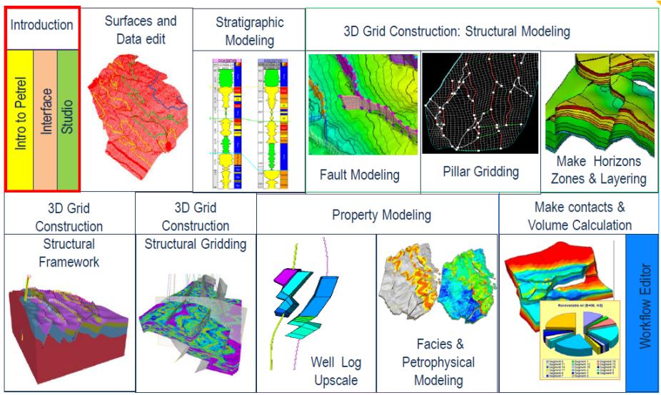Figure 1: Steps of 3D modeling of GD reservoir [10]

3.2.1 Structural model

a. Fault model

Seismic interpretation results show that field DH area has a complicated fault system with 3 main directions: Northeast-Southwest (NE-SW) (300 and 450), Northwest-Southeast (TB-SE).) and sub-latitude. The fracture system in NE-TN 300 direction has a large displacement and length, determines the structure of the field, while the systems of NW-SE direction and sub-latitude are not large in length, with small displacement amplitude. plays the role of dividing the field into smaller structural zones.

At field DH, dozens of faults have been explained and mapped. However, within the scope of the thesis, the author has selected 4 main faults, which are 4 blocking faults of the F block area.

The fracture pattern is properly tested for the litric fracture type, the shape of the fracture must match relatively exactly with the original input, ensuring the faults are connected at the intersection of the two fractured, where the contact between the cartilage wing and the lift wing.

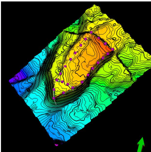Figure 2: Complete fault model

b. Grid model

The grid model must have a grid size that is small enough to represent the reservoir's characteristics and the quantity is not too large due to the limitations of the computer hardware. Normally, the grid size is chosen to be 25mx25m; 50mx50m or 100mx100m respectively for small and larger model area.

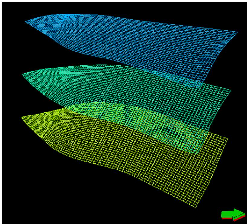Figure 3: Model of a complete grid in the 3D window

For block F of field DH, the selected grid is 25mx25m (IxJ). Then using three large faults to make boundary for the block, simultaneously dividing 2 segments to divide the seam's fluid bond for more accurate reserve calculation.

c. Structural model

☐ Modeling of stratigraphic surfaces (Make Horizone)

The main structural layer is modeled on the basis of the isometric structure map from seismic explanation results. Then it combined with the results of the division of the top and bottom of the reservoir from the well log interpretation and the well markers are adjusted to match the top and bottom map of the Miocene set. The amplitude of the lateral displacement of the faults is adjusted for each fracture on the surface.

By using the Make Horizon function in Petrel software, building 6 main structure layers based on the isometric structure map, including: H95, H100, H125, H140, H145, H150.

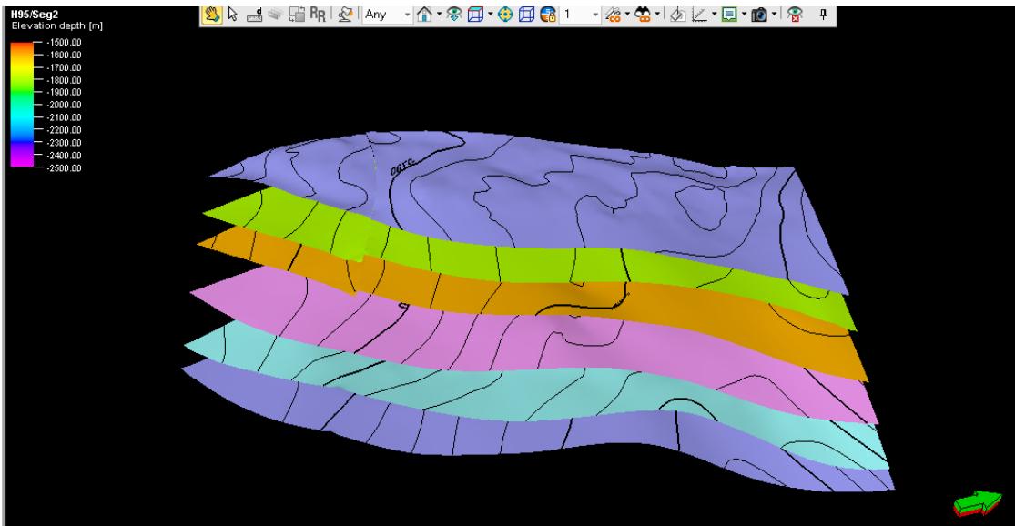Figure 4: Model of main structural layers, block F, field DH

☐ Modeling containing reservoir and dividing layers (Make zones and Layering)

The reservoir are modeled based on the model of main reservoir which is newly built; combined with the results of dividing the top and bottom of the reservoir from the well log interpretation, the pressure document and the connection through the wells.

The results of the interpretation of the pressure along the well show that the product in the block area F, field DH are a multistage reservoir system, hydraulically different from each other in the vertical direction.

The division of top and bottom of the reservoir is mainly conducted on the variation of the natural radiation curve (Gamma Ray) combined with the results of the pressure explanation. These reservoir will then be linked between wells in the block and through blocks on the basis of a synthesis of research results on stratigraphy, stratigraphy... and especially the pressure relationship between the wells. Results of the division of the top and bottom of the reservoir for Miocene aquifer under block F are shown in Figure 5 below.

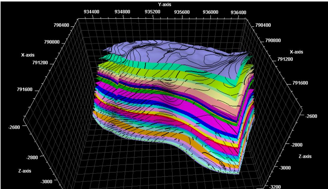Figure 5: 3D Modeling containing reservoirs and dividing layers of block F

3.2.2 Facies model

Because field DH area is in the mining phase, the parametric models must be built in more detail to show the petrographic properties of the reservoir most closely. Therefore, building rock facies model is not merely simulating two types of containment and non-containment rock, but must be modeled in different way to reflect more clearly the connection of the oil bodies, as well as the heterogeneity of containing layer.

The results of environmental interpretation from the core sample document show that there are more than ten types of rock facies belonging to the river/lake environment identified in the study area. However, it is difficult to be able to predict these types of facies in the core sampling spaces at drilled wells and then to simulate the strata according to the Depositional Facies model. Therefore, it is still simulating the reservoir according to the litho facies including containing rock and non-contain rock but dividing the reservoir rock into different types of HFU (Hydraulic Flow Units) based on their porosity properties on the basis of Core sample analysis results were used in the facies modeling step.

Model of containing rock distribution according to each HU types is rarely used in oil and gas fields in Vietnam. The advantage of this method is that it reflects quite clearly the level of heterogeneity of the containing rock distribution, the petrographic physical parameters, especially the permeability parameter. Although there are significant advantages, the prediction of rock facies distribution outside the well location still has certain limitations and needs to be verified by new wells.

According to the convention that applies to the majority of oil fields around the world, the critical value for permeability for terrigenous sandstone reservoir, is 1mD. Rock with a permeability of less than 1mD will be considered impermeable. From the results of core samples analysis taken from the wells, effective porosity ( ), permeability (K) values, the corresponding RQI (Reservoir Quality Index) and FZI (Flow Zone Indicator) values are calculated on the basis of the following equations:

In which:

These newly calculated FZI values will be plotted by statistical probability to determine the number of HU from core sample analysis document. In Figure 6, it is possible to group containing rocks into 4 types HU corresponding to 4 lines with different slope angles representing each type of HU.

Base on the results of dividing the containing rock into 4 HU according to the core sample document just mentioned above, combined with the geodetic curves such as GR, deep resistance, density, neutron, ultrasound, using ANN method in IP software to predict FZI values and then group by HU type for the spaces without core samples in the entire slice of wells according to the following steps:

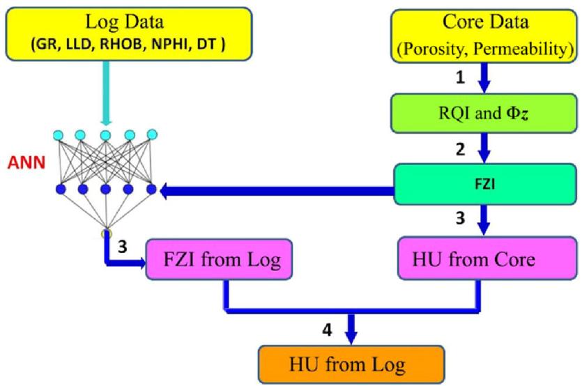Figure 7: HU classification process

After identifying each HU type in each A-12P, 13P and 24XP cut section according to the above procedure, they will be shown on the well link cross section for correction if necessary. From Figure 7 it can be seen that HU1 corresponds to clay (not contained), HU4 corresponds to the reservoir with the highest porosity.

The HU curves will then be averaged onto the grid as input for the rock facies modeling (Figure 8).

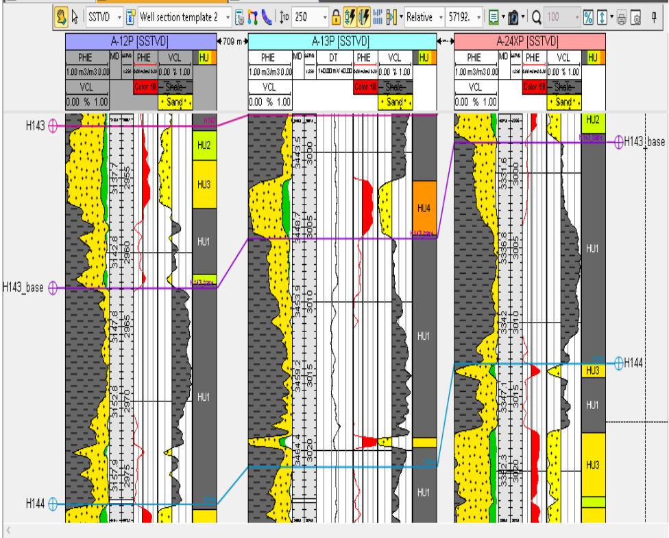3D 3D window 1 [Any] ✗ Well section window 1 [SSTVD] ✗ 2D 2D window 1 [Any] ✗

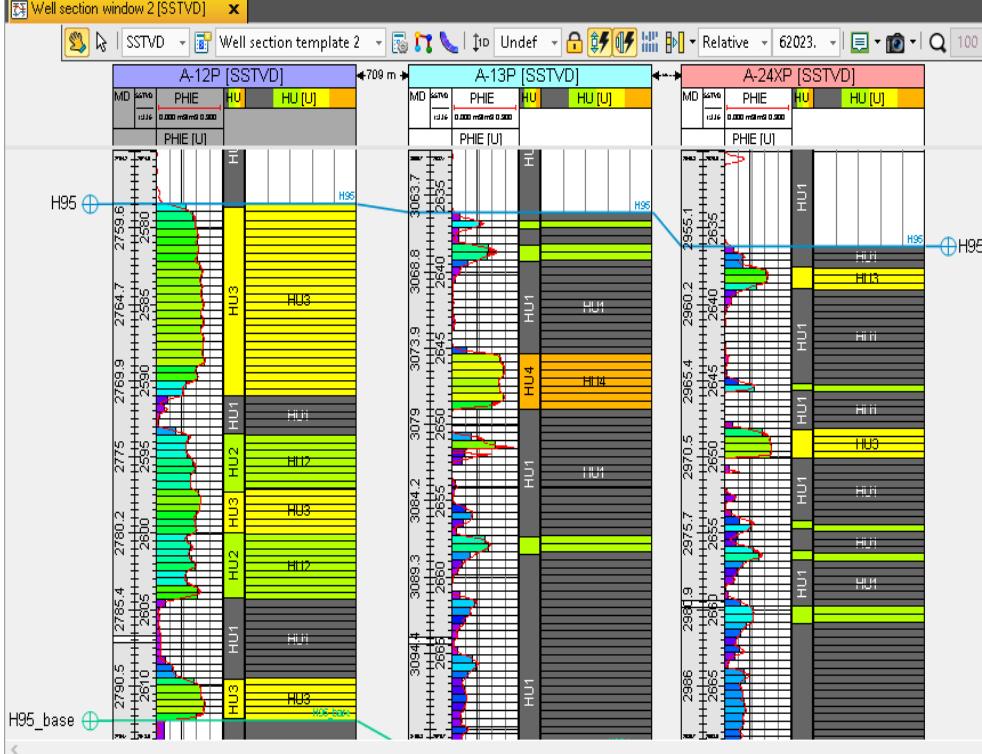Figure 8: HU types at field DH

Base on the normalized rock facies (HU) curves, the model of rock facies distribution of the lower Miocene, block F, field DH will be simulated according to each HU type using random simulation method according to SIS algorithm.

Comment on facies model

Using SIS method to construct the facies model for block F gives rapid simulation results and is suitable with the well data because of the constraints with the input data. The chart shows that there is a small variation of the general model before and after simulation, the error is within an acceptable range (less than 5%).

3.2.3 Properties model

a. Porosity

The porosity is measured from well log interpretation, then averaged and modeled by Gaussian Random Function Simulation. By using parallel kriging theory, the GRFS method produces more accurate results and saves model runtime.

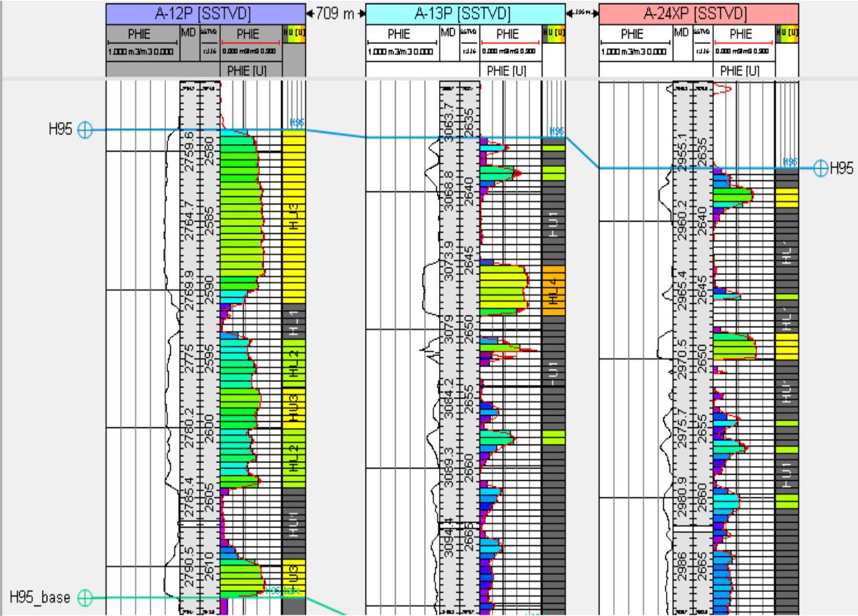Figure 9: The results averaged HU

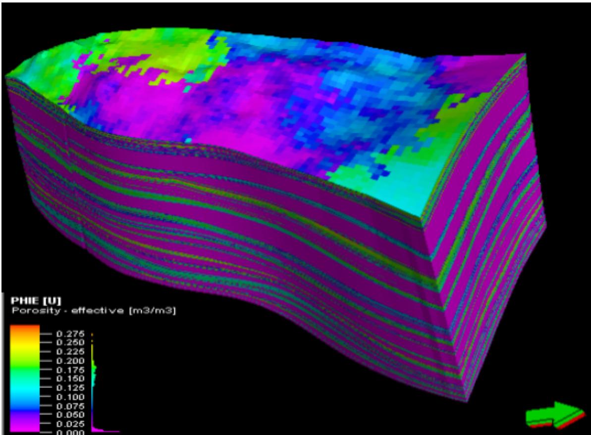Figure 13: Complete porosity model

Comment of porosity model

By using the GRFS method, the porosity model of block F showed clearly the distribution of fluid capacity according to the data trend. From the model, we can see that the porosity distribution is reasonably variable, not suddenly dispersed, ensuring the validity of the model; the chart showing the variation of the data before and after the simulation has not too large error, ensuring model reasonableness.

b. Permeability model

Based on the porosity-permeability relation function obtained from core sample analysis, the permeability is modeled by Gaussian Random Function Simulation, similar to the porosity.

The permeability functions are built for 4 different porosity ranges according to the following equations:

HU1 and HU2:

HU3:

HU4:

is porosity from model (%).

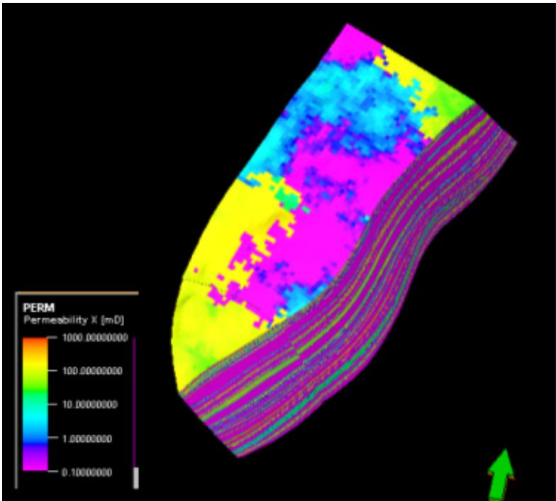Figure 14: Permeability model

Comment on permeability model

Permeability model is based on porosity-permeability relation function, ensuring consistency with porosity distribution. High permeability correspond to the good porosity facies (HU3, HU4), low permeability is correspond to appearance shale (Non - reservoir) with poor porosity.

c. Saturation model

Water saturation is averaged and simulated by sequential Gaussian simulation (SGS).

The water saturation (Sw) model is simulated using the function of water saturation with the height of the oil body (h) above the free water boundary (High above contact) and the model of permeability distribution. The functions of saturation are built for 4 different porosity ranges according to the following equations:

HU1 and HU2:

HU3 and HU4:

In which: Sw is the water saturation (%);

HAC is the height of oil body (m);

K is permeability (mD);

is the porosity from the model (%).

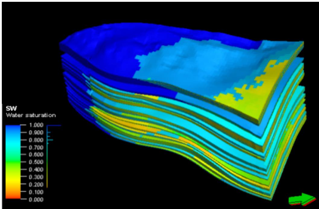Figure 16: Water saturation model

Comment on saturation model

The water saturation model based on the height-function from core sample analysis gives more reliable results than the water saturation model based on interpretation results from the well.. Modeling of water saturation based on saturation pressure, surface tension,... clearly shows the height of the transition zone between the oil-water boundary.

Based on the facies model and the newly porosity and saturation parametric models, oil reserves in place will be calculated using the Volumetric Calculation function:

Therefore, oil reserves in place of block F, field DH according to the model is bbl.

3.3 Sensitivity Analysis

Sensitivity analysis is often performed to better understand the effects of variables or parameters about the distribution of uncertainty.

Sensitivity analysis is analysing the effects of input uncertainties (in this case: storage volume, ratio of effective and total thickness, porosity, water saturation, formation volume factor) to the output (oil reserve in place). In other words, sensitivity analysis considers the sensitivity of the results to a change of an input value.

Within the paper, the author performed a variable sensitivity analysis (Uncertain, SEED), set up a loop so that the variables were randomly taken in the range from 10,000 to 100,000.

All important parameters such as Facies modeling and Petrophisical modeling are taken to calculate for each respective seed.

The larger the number of scenarios, the higher the confidence level. However, the number of possible scenarios depends on the computer configuration. Here, the author has run 50 scenarios.

It can be seen that, the results of assessing oil reserves in place according to the model of the author (46.0585 106 bbl) compared with the uncertainty results at P50 (45.7259 106 bbl) have an error of 0.72%. \<5%, so reliability of the model is acceptable.

IV. CONCLUSION

The three-dimensional geological model of terrigenous sandstone reservoir, block F, field DH, is built by geostatistical algorithms. Based on the geological features of field DH as well as input data, the stochastic method was used to represent the heterogeneity then provide attribute models. The lithological method of flow monomorphic analysis helps to divide stone facies based on their capacity. The advantage is to reflect the degree of heterogeneity of the containing rock distribution and the petrographic physical parameters, especially the permeability parameter. The GRFS method saves simulation time and gives more accurate results than the traditional SIS method thanks to the application of the parallel Kriging algorithm. Base on the geological model, it clarifies the origin of lithological facies and distribution of porosity, permeability, NTG, etc. Then evaluating oil reserves based on Petrel software to give the development project.

Accordingly, the facies model, the random models of the porosity, permeability and water saturation all show similarities of the general trends in the reservoir. The containing layer of field DH has good quality, reflected in porosity, high NTG, and low water saturation.

The process of checking the accuracy of the model is conducted by comparing data from the probability model and input data, ensuring that it does not exceed the allowable limit (\<10%).

Model uncertainty depends on many different factors, which can be attributed to: reservoir structure, fluid boundary, uncertainty in facies model and properties model, Bo parameter. The importance of research papers about sediment environments or data for facies modeling was confirmed through analysis of the influence of the component models and experience of model constructor. According to the author, the most important factor is the error when construct the models. In addition, the computer configuration of each performer should also be mentioned.

ACKNOWLEDGEMENT

This research is funded by Ho Chi Minh City University of Technology - VNU - HCM under grant number To-DCDK-2019-24.

Conflicts of interest/ Competing interests

I guarantee that there is no conflict of interest between the authors and sponsors.

{"image_source":{"path":"images/f08f6f937a926829ff7b6f9c837fdc01769b0adcdf511f3306b33e684b22bbb7.jpg"},"content":"","chart_caption":[{"type":"text","content":"Figure 6: Determine the HU quantity based on the core sample document"}],"chart_footnote":[]} {"image_source":{"path":"images/45eccfd38efbf42273c93cda07ab0437251cbb9fe83b051f17e7b1676818e8c0.jpg"},"content":"","chart_caption":[{"type":"text","content":"Figure 10: Rock facies before and after the simulation"}],"chart_footnote":[]}

{"image_source":{"path":"images/d4b03bd66b9574430c76409afe49c9a99cce5421f5272dd7eeb1ac425008cb0c.jpg"},"content":"","chart_caption":[{"type":"text","content":"Figure 11: The results of porosity after being averaged"},{"type":"text","content":"Figure 12: Comparison of porosity parameters before and after the simulation"}],"chart_footnote":[]} {"image_source":{"path":"images/e860afecf31c21dd2c62714bca4a80a449e0910ad63a829c1e56380dc8b9d7cd.jpg"},"content":"","chart_caption":[{"type":"text","content":"Figure 15: Permeability distribution range."}],"chart_footnote":[]}

{"image_source":{"path":"images/23d325fad9f890545a45df8ff7baf1e257284ffd4c5ce89a6141e97e1672d390.jpg"},"content":"","chart_caption":[{"type":"text","content":"Figure 17: The distribution of water saturation"}],"chart_footnote":[]} {"image_source":{"path":"images/936ed78ba6c8dd6724214fa5191ddaa6e2b4e0a74475fd312cd7c74d351a80c5.jpg"},"content":"","chart_caption":[{"type":"text","content":"Figure 18: Result of oil reserves of block F, field DH"}],"chart_footnote":[]}

{"image_source":{"path":"images/4ba72cb9eec48e089a8f737ca15cec5bfb69484ffea711dc1347518103868336.jpg"},"content":"","chart_caption":[{"type":"text","content":"Figure 19: The results of reserves for over 50 scenarios."}],"chart_footnote":[]}