


IntelliPaper
Abstract
X-ray diffraction (XRD) plays a pivotal role in material characterization, offering valuable insights into crystalline structures. This study introduces a comprehensive framework for autonomous phase identification through a machine learning-guided approach. The proposed methodology comprises four key stages. In the pre-processing phase, raw data undergoes meticulous cleaning to eliminate noise, followed by normalization and smoothing procedures to ensure data integrity. Feature extraction involves a multi-faceted approach. Peak identification meticulously captures critical features such as peak position, intensity, and width within XRD patterns. Statistical features, encompassing mean, standard deviation, skewness, and kurtosis, provide a robust characterization of the dataset. The incorporation of Discrete Wavelet Transform further enriches the feature space by capturing both high and low-frequency information. For feature selection, a Hybrid Optimization Approach, combining the Kookaburra Optimization Algorithm (KOA) and White Shark Optimizer, is employed. This ensures an optimal subset of features for subsequent analysis. Phase identification is facilitated by a Bayesian FusionNet, integrating the strengths of Improved GhostNetV2, Bayesian Neural Network (BNN), and Feedforward Neural Network (FNN). The outcomes from these models are aggregated by taking the mean, enhancing the reliability and accuracy of phase identification. This innovative framework not only automates phase identification in X-ray diffraction but also showcases the efficacy of a hybridized machine learning approach, amalgamating optimization algorithms and neural networks for enhanced performance and interpretability. The proposed methodology holds significant promise for advancing material science research and facilitating efficient analysis in diverse applications.
Explore Digital Article Text
I. INTRODUCTION
An XRD is a useful non-destructive analytical technique for analyzing crystal structure, phase composition, and orientation of powder, solid, and liquid materials . Tiny crystallites include a wide variety of materials. The term "phase" refers to these crystals' structural type and chemical makeup. Materials may consist of both crystalline and non-crystalline components, and they may be single phase or multiphase mixes . An X-ray diffractometer can distinguish between different crystalline phases by their respective diffraction patterns . Phase identification is often carried out by comparing reference database patterns to X-ray diffraction patterns acquired from unidentified materials. This method is comparable to the procedure of comparing fingerprints at a crime scene . XRD is the result of constructive interaction between crystalline sample and X-rays. The wavelength of the X-rays used is equal to the distance between atoms in crystalline lattice . The resulting diffraction pattern may be analyzed in several ways, most popular being the application of widely recognized Bragg's Law, which is used to measure crystals and their phases . An X-ray source, XRD detector, and sample container are the three main parts of X-ray apparatus. X-rays that the source emit light the sample. After that, sample phase diffracts it so that it may get into detector . Adjusting sample, tube, and detector to change diffraction angle determines the intensity and collects diffraction data. Depending on sample type and diffractometer's geometry, the angle between incident beam and sample can be either constant or variable and is commonly matched with diffracted beam angle .
Algorithms for machine learning are ideal for analyzing big and complicated datasets because they can recognize patterns and correlations in the data. They have been used in materials research to solve a variety of issues, such as the processing of imaging data and the prediction of material characteristics . Machine learning has been applied to X-ray diffraction for the purpose of classifying diffraction patterns and analyzing crystal structure . An interpretable machine learning model can enable data-driven quantification of empirical expert knowledge, and a quick and easy machine learning approach can categorize crystal systems and space groups based on powder XRD patterns with high accuracy. The powder XRD pattern need to be employed as material descriptor for machine learning (ML)-based symmetry detection and property prediction . Recent years have seen a major increase in the interest of material scientists and engineers in machine learning as well as high-throughput testing and computation. It is common practice to create suitable material descriptors for the systematic representation of materials in prospective machine learning models . As long as actual or theoretical standard powder XRD patterns are available, knowledge-based material descriptors cannot be extracted for use in ML . Full-profile powder XRD patterns, which indicate the material identity, may be used in place of conventional descriptors that need complex knowledge-based extraction processes. It is difficult to create a flexible ML model that can predict properties and identify symmetry for all typical inorganic materials . The incorporation of ML techniques into XRD pattern analysis has been driven by need for accurate phase identification, quantification of multiphase mixtures with varying raw data quality, and expansion the amount of data that is available . Processing XRD observations has become increasingly dependent on ML over past 10 years as processing power has increased and both XRD and ML have been made simpler and better.
This study introduces a novel framework for autonomous phase identification in XRD, leveraging a hybrid approach that combines feature-optimized ensemble learning with a Bayesian FusionNet. The primary aim of this research is to develop a self-sufficient method for phase detection in XRD by utilizing machine learning and optimization approaches. Beyond simple automation, a hybrid technique combining the best aspects of feature-optimized ensemble learning and Bayesian FusionNet is being researched and developed.
1.1. Contribution of Study
The following is an overview of the study's contributions:
The paper discusses the necessity of automating the X-ray diffraction phase identification procedure. The paper contributes significantly to simplifying XRD pattern analysis, which is essential for material characterization, by presenting a complete framework incorporating machine learning-led techniques.
The use of a Hybrid Optimization Approach, combining the Kookaburra Optimization Algorithm (KOA) and White Shark Optimizer for feature selection, is a notable contribution. By doing this, the efficiency and efficacy of the phase identification process are maximized since the most pertinent subset of characteristics is chosen for further examination.
Phase identification is made more accurate and reliable by using ensemble learning, namely by averaging the results from Improved GhostNetV2, BNN, and FNN. An improved forecast is produced by using ensemble approaches, which lessen the biases and mistakes of individual models.
The suggested approach has plenty of potential for developing material science research. The study enhances an efficacy and efficiency of material analysis by automating and improving phase identification procedure in XRD.
1.2. Structure of Paper
The remaining part of paper is structured as follows: In Section 2, relevant existing works are provided; proposed methodology is covered in Section 3; Section 4 provides an explanation of the findings; Finally, Section 5 includes a conclusion and suggestions for further research.
II. LITERATURE REVIEW
The study of literature provides an extensive overview of what is currently known about autonomous phase identification in X-ray diffraction. By laying out the background, offering a historical viewpoint, and critically assessing the most recent approaches, it prepares the reader for the later sections of the work. In the end, it justifies the novelty and applicability of suggested hybrid approach using Bayesian FusionNet and Feature-Optimized Ensemble Learning.
In 2020, Hocine et al., [16] described the application of operando X-ray diffraction in laser-assisted 3D printing. Operando X-ray diffraction, according to authors, is a method that enables real-time observation of structural alterations that take place during printing. To optimize the printing settings and raise the caliber of printed goods, the study emphasized how crucial it is to comprehend these alterations. Operando X-ray diffraction can offer insightful information about the printing process and help enhance 3D printing technology, according to conclusion.
In 2019, Oviedo et al., [17] presented a novel approach that makes use of deep neural networks and data augmentation to identify tiny X-ray diffraction datasets. This study provided a quick and easy-to-understand method that raises classification accuracy. This paper identified potential differences between experimental thin film XRD patterns and simulated XRD powder patterns by proposing a physics-informed strategy for data augmentation that expands limited, focused experimental and simulated datasets. The process entails training a deep neural network to categorize the diffraction patterns and artificially growing dataset using data augmentation techniques. The efficiency and precision of X-ray diffraction analysis in materials science research may be improved by using this method.
In 2020, Lee et al., [18] presented a simple, quick methodology based on deep learning methods to solve complicated multiphase inorganic compound challenges including phase identification and measurement. A viable powder XRD pattern simulation was performed on 170 inorganic compounds in Sr-Li-Al-O quaternary compositional pool, where potential LED phosphors have been discovered. Finally, 1,785,405 synthetic XRD patterns were produced by combinatorially merging simulated powder XRD patterns of 170 inorganic compounds. This large prepared dataset was used to build and train convolutional neural network (CNN) models. The fully trained CNN model accurately and rapidly detects component phases while working with complex multiphase inorganic substances.
In 2022, Sivaraman et al., [19] addressed the difficulties in figuring out relationships between structure and properties of amorphous and liquid metal oxides. This study was suggested predicting chemically realistic structures for by ML with Gaussian Approximation Potential (GAP). The GAP model used training datasets to achieve Density Functional Theory-Strongly Constrained and Appropriately Normed (DFT-SCAN) theoretical level. This topology was shown to be consistent with structure of a range of liquid and amorphous transition metal oxides with different ion sizes, including TiO2 and ZrO2.
In 2020, Utimula et al., [20] highlighted the use of ML clustering to analysis of powder XRD pattern to determine ThMn12-type alloys of compositions. This paper investigates the potential applications of this method to further materials science's knowledge of alloy composition. The XRD spectrum patterns are subjected to a clustering approach employing dynamic-time-wrapping (DTW) analysis to determine microscopic structures of substituents added to main phase of magnetic alloys. This methodology developed here was not exclusive to system under consideration; rather, it may be broadly applied to systems whose attributes are to be adjusted by atomic replacements within a phase.
In 2022, Dong et al., [21] delivered a deep learning algorithm that can be used to predict XRD spectrum based only on a material's composition. This algorithm can then be used to infer important structural features for structural analysis that occurs later on, such as classification of crystal systems or space groups, calculation of crystal lattice parameters, or prediction of material properties. This DeepXRD algorithm may obtain good performance for XRD prediction as assessed across test sets according to benchmark tests on two datasets. Therefore, it may be applied to high-throughput screening for identification of novel materials in the vast materials composition space.
In 2023, Utimula et al., [22] designed autoencoder to build a feature space describing XRD patterns. In this paper, the training of an autoencoder to detect systematics resulting from atomic changes inside single phase without structural transitions was presented. The trained autoencoder builds a feature space that correctly identifies substitution compositions of XRD patterns. A projected XRD pattern to a point and compositions interpolated in feature space coincide rather well. After that, interpolated point in feature space is used by autoencoder to create a virtual XRD pattern. When feature space was effectively tailored by enough training data, the autoencoder predicts an XRD pattern with concentration that is difficult to quantify using potential resolution of supercell technique of ab initio calculations.
In 2022, Massuyeau et al., [23] established a machine learning-based method that uses powder X-ray diffraction patterns to automatically identify if an unknown substance is a perovskite type. RF and CNN models were used to identify the different perovskite structure types based on the hybrid lead halide powder X-ray diffraction patterns. The structural types of novel unknown compounds might be predicted from their experimental powder XRD patterns once a deep learning network had been trained on a dataset of known compounds. In an array of novel hybrid lead halides, this technique was employed to discern perovskite-type materials.
In 2021, Banko et al., [24] Applied variational autoencoders (VAE) to analyze thin-film data from experiments and simulations for XRD. The structural similarity of textured diffraction patterns is one example of latent information that may be revealed by using crystal structure representations that a VAE has learnt. Although other artificial intelligence (AI) agents are effective in classifying XRD data into known phases, similarly conditioned VAE excels at understanding what it does not know. It can identify novel phases and blends, as well as data outside the distribution it was trained on, very rapidly. These characteristics highlighted the value of VAE as an AI for deciphering XRD data and supporting materials discovery both "on the fly" and during post hoc analysis.
In 2020, Wang et al., [25] presented a convolutional neural network (CNN) model that uses sparse experimental data to quickly identify metal-organic framework (MOF) XRD patterns. The noise collected from experimental spectra was added to theoretical data to train the model. The investigation additionally examined the CNN model's activation properties using class activation maps (CAMs) and utilized neighbourhood component analysis (NCA) to cluster XRD data from the same MOF. The potential of CNNs for individual material identification is demonstrated by this work.
2.1 Problem Statement
The statement of problem emphasizes how important it is to develop phase identification techniques to stay up with the increasing diversity and complexity of materials under study. X-ray diffraction analysis might undergo a revolutionary change with the help of this hybrid solution that attempts to close the gap between conventional methods and the rapidly changing area of machine learning. Table 1 illustrates the features and limitations of various existing techniques.
| Author | Method | Features | Challenges |
| [16]Hocine et al., 2020 | operando | The laser settling time may be ascertained with this experiment. | This approach becomes particularly critical for modeling tiny structures. |
| [17]Oviedo et al 2019 | physics-informed data augmentation | ·Accessible assessment of errors.·A technique for augmenting data that facilitates quick and precise categorization. | The framework may be expanded to include any spectrum with information-rich characteristics that need to be classified, in addition to XRD classification. |
| [18]Lee et al 2020 | CNN | ·Recognizing the many stages of inorganic multiphase structures.·Observe trends and formulate forecasts. | It is not applicable to highly entropy systems. |
| [19]Sivaraman et al 2022 | ML with GAP | It offers a way to generate an ML-IP with ab initio accuracy by directly validating model during active learning process. | Long-range electrostatics must be explicitly included in modeling of non-isotropic chemical environments |
| [20]Utimula et al 2020 | DTW | ·Differentiate between substituent concentrations.·The predictive power of framework is higher. | The contraction causes a shift in peak locations, which is not picked up by system. |
| [21]Dong et al 2022 | DeepXRD | ·Research using two datasets as benchmarks to assess performance.·Examination of potential for XRD spectrum prediction. | ·It is expensive to experimentally characterize crystal structures using XRD.·Restricted to rather small systems; it is not suitable for extensive screening. |
| [22]Utimula et al 2023 | Autoencoder | ·Determining doping levels.·Elucidating pointlessness of each top.·Producing synthetic XRD patterns. | It was unable to provide a plausible explanation for XRD's physics-related irrelevance. |
| [23]Massuyeau et al 2022 | RF and CNN | ·Automatically identify the perovskite type of a given material.·It had the capability to forecast the kinds of | Powder XRD patterns could not distinguish between perovskites and non-perovskites without laborious structural determination. |
| structures of novel, unidentified chemicals. | |||
| [24] Banko et al 2021 | VAE | · It may be applied to real-time examination of distribution of dataset among several structures. | veracity and efficacy of high-throughput diffraction must be increased. |
| [25] Wang et al 2020 | CNN | · Observed that the presence of noise and reduced crystallinity had a significant impact on categorization accuracy. | The identification of individual XRD patterns from a large database of spectra is a challenging task. |
III. PROPOSED METHODOLOGY
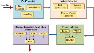
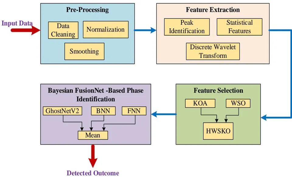
This study proposes a novel and complete framework for autonomous phase identification in XRD, using ML-guided approaches for improved interpretability and accuracy. There are four main phases in this technique, and each one adds to the overall stability and effectiveness of the phase identification process. Pre-processing (data cleaning, normalization, and smoothing), feature extraction (peak identification, statistical features, and discrete wavelet transform), feature selection (via a hybrid optimization approach utilizing Kookaburra Optimization Algorithm and White Shark Optimizer), and Bayesian FusionNet-based phase identification (combining Improved GhostNetV2, Bayesian Neural Network, and Feedforward Neural Network, with results aggregated by taking the mean) are the four essential stages. This novel method of automating phase identification demonstrates the convergence of neural networks, optimization methods, and machine learning. The approach is a potent tool for scholars and practitioners, with the potential to further material science research and enable effective analysis in a range of applications. The advancement of material characterisation techniques is facilitated by the combination of various approaches, which improve phase identification efficiency, interpretability, and reliability. The proposed architecture is displayed in Fig. 1.
3.1. Preprocessing
Pre-processing for Autonomous Phase Identification in X-ray Diffraction is a method that makes use of machine learning to help with and enhance material characterisation. This makes it possible to automatically interpret experimental data using methods like XRD. This technique combines analysis and diffraction such that measurements are guided toward characteristics that raise confidence of model that has been trained for recognize crystalline phases. This allows for utilization of early experimental data. The methodology entails integrating a physical diffractometer with an ML algorithm to facilitate the detection of transient intermediate phases generated in solid-state processes on-site, utilizing a standard diffractometer located within the organization. Accurate identification of minute quantities of components in multi-phase mixtures at short measurement durations is also made possible by the faster phase detection process. The preprocessing stage includes data cleaning, normalization, and smoothing.
A. Data Cleaning
The process of eliminating or rectifying outdated, inadequate, or incorrect information from the raw diffraction pictures is known as data cleaning in X-ray diffraction preprocessing. This procedure is necessary because the precision and dependability of the structure determination are greatly impacted by the quality of the data utilized in X-ray diffraction. The following are a few of the procedures in data cleaning for X-ray Diffraction preprocessing:
i. Spot finding: This process eliminates any background pixels and noise by locating and determining the strengths of the diffraction spots on each image.
ii. Indexing: In this stage, each spot is given a distinct set of three integers, or Miller indices, based on experimental setup.
iii. Parameter refinement: This stage determines the estimated errors associated with each reflection's integrated intensity, which is the total of all the spots' intensities that correspond to the same reflection.
iv. Integration: The integrated intensity of each reflection, which is the total of the intensities of all the spots that belong to the same reflection, is calculated in this phase along with an estimation of the related errors.
v. Scaling and Merging: This process merges the data from multiple images into a single dataset and corrects the intensity data for a number of variables, including absorption, polarization, and exposure duration.
B. Normalization
A technique for data processing called normalization seeks to lessen the impact of artifacts and intensity variations in XRD patterns. Phase identification, peak fitting, and structural determination are few of the XRD analyses that can benefit from normalization's increased precision and dependability. The category and source of XRD patterns determine which normalization approach is used for XRD data. Some of the most popular techniques for normalizing are:
i. Normalization by the background intensity: The measured intensity is divided by the background intensity, which may be calculated by fitting a polynomial or spline function to the XRD pattern's baseline. This approach accounts for fluctuations in background noise and artifacts. Applications of this technique include micro-XRD patterns obtained from liquid phase in-situ studies.
ii. Normalization by the total scattered intensity: The measured intensity is divided by the total scattered intensity (which may be computed by integrating the complete XRD pattern) in this approach to account for differences in sample transmission and absorption. This technique works well with ultrafast XRD patterns obtained from thin-film materials utilizing a plasma source powered by a laser.
iii. Normalization by the incident beam intensity: The incident beam intensity, which can be seen by a beam stop or a reference detector, is divided by the measured intensity in this technique to account for fluctuations in the X-ray source intensity. Conventional XRD patterns obtained from solid materials in an ambient setting can be used with this approach.
Normalization is a crucial preprocessing procedure for XRD data since it improves the comparability of various XRD patterns and the signal-to-noise ratio. Normalization can also help with application of ML methods for XRD data interpretation.
C. Smoothing
Data noise is minimized by the use of digital filter smoothing, also known as Savitzky-Golay smoothing. The application uses the variance approach to assess the amount of noise in the pattern and automatically modifies the smoothing settings based on that level. Different smoothing parameters are employed for the crystalline and amorphous components of the pattern, if the user chooses to match them (for the amorphous instance, often more smoothing is applied).
3.2. Feature Extraction
A crucial part of medical image analysis is feature extraction. From the previously processed data, features are extracted. The process of converting pre-processed XRD data into a more compact and useful representation that can be utilized for additional analysis is known as feature extraction. This stage includes peak identification, statistical features, and discrete wavelet transform.
A. Peak identification
The technique of identifying the distinctive peaks in an X-ray diffraction (XRD) pattern that represents a material's crystal structure and content is called peak identification. It is possible to extract and use as features for a variety of studies the peak position, intensity, and width of these peak.
i. Peak Position: The peak position (also known as the diffraction angle) depends on separation between reflection planes when wavelength is constant. Consequently, the distance of peak location and reflection plane coincide. Peak location is often determined using following techniques:
Estimating peak position directly from angle of diffraction.
Calculating peak position using maximum angle after smoothing.
Using mathematical functions fitted to measured line.
ii. Peak Intensity: The maximum intensity is height at which an XRD peak is at its highest point. Frequently, it lines up with height at Bragg's angle. The geometric relationship between an XRD peak's total intensity and HW, Imax, and Sc is as follows:
Where,represents raw intensity of XRD;is a physical constant;denotes weight fraction;means temperature factor;represents multiplicity factor; volume of unit cell is denoted by;stands for density;represents modulus of amplitude scattering in the direction of angle;represents distribution factor;symbolizes mean mass absorption coefficient;is shape of SRD peak; HW means width at half maximum intensity.
iii. Width
Divergence magnitude is dictated by the aperture of the divergence and the effective focal width of the source. The mathematical formula of maximum width is given in following Eqn. (2)
In above equation, width is represented by W; K denotes constant; represents wavelength; denotes diffraction line.
B. Statistical Features:
i. Mean: The arithmetic average of the data set is calculated using the mean. It refers to the total number of values divided by the sum of all the values. The mean is quite simple. Its estimation of the data values is excellent.
ii. Standard deviation: This is a statistical technique used to measure degree of dispersion or variation for a set of data points. When describing spread or breadth of diffraction peaks in an XRD examination, the standard deviation is frequently employed to provide details about the homogeneity and crystalline quality of a material.
iii. Skewness: Skewness quantifies how dissimilar a real-valued random variable's probability distribution is from one another. The skewness can be calculated using following Eqn.
iv. Kurtosis: Kurtosis is a statistical metric that quantifies the peak or flatness of a real-valued random variable's probability distribution. The following equation can be used to determine the kurtosis.
Where, n represents number of data; denotes individual data; is mean of data; standard deviation of data is represented by SD.
C. Discrete Wavelet Transform
A mathematical method known as the Discrete Wavelet Transform (DWT) can divide a signal up into its frequency components. Wavelet transform uses a series of basic functions, termed wavelets, which are scaled and shifted replicas of a mother wavelet to capture both high-frequency and low-frequency information. The wavelets are limited in duration and can adjust to the specific characteristics of the signal locally. At every stage of decomposition, the DWT processes the signal through a number of filters to provide a comprehensive information at each level as well as a coarse approximation. The low-frequency information is contained in coarse approximation, while high-frequency information is contained in detailed information. The DWT may be utilized for variety of tasks and applied to wide range of data kinds, including vibrations, images, and noises.
DWT may be practically implemented using two filters: one for low-pass and one for high-pass. Wavelet dilation and shifting operations are used to create a wavelet of a prototype signal, sometimes referred to as a "mother" or "single modeling" wavelet y (t). The following formula illustrates this connection.
Where, j represents scaling factor; t denotes time; k is shifting parameter; denotes function of mother wavelet; DWT may be calculated mathematically by convolving the signal with the mother-wavelet dilated, reflected, and normalized. The mother-wavelet convolution of the data gives Equation (8).
The signals are broken down by filters into approximation and detail coefficients, whose computation is given as
The aforementioned equations may be more precisely described using following convolution technique that stated in Eqn. (11) and (12).
The high-frequency and low-frequency components are represented by the low- and high-pass filters in equations (9) and (10) respectively. The outputs provide the approximation (from the low-pass filter) and detail (from the high-pass filter) coefficients. Fig. 2 depicts the 2-level DWT decomposition process.
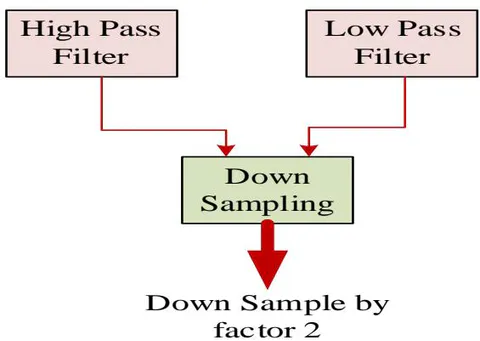
The patterns of diffracted X-rays from a crystalline material can be examined using DWT in XRD. The phase composition and crystal structure of material are disclosed using XRD data, which may be seen as 1D signal. It may be divided into several frequency bands that correlate to various spatial scales of crystal lattice by DWT on XRD data. The overall phase composition and average lattice parameters are revealed by low-frequency bands, and crystal structural and local fluctuations defects are shown by high-frequency bands. It is also possible to identify and quantify the diffraction peaks more easily using DWT to lower noise and improve peaks and in XRD.
3.3. Feature Selection
Feature selection is a method of reducing dimensionality strategy that selects a subset of useful characteristics by eliminating noisy, redundant, or irrelevant features from the original set. Feature selection frequently leads to higher learning accuracy, increased model interpretability, and lower processing costs. It is possible to reduce data effectively by using feature selection techniques. This helps locate precise information. Feature selection can reduce measurement and storage requirements, training and utilization durations, and curse of dimensionality to improve prediction performance. It can also help with data presentation and interpretation.
In feature selection, hybrid optimization is a methodology that combines many approaches to improve efficiency and performance. In this study, Hybrid White Shark Optimizer and Kookaburra Optimization Algorithm (HWSKO) is introduced to provide effective feature selection. It is a novel feature selection method that combines the advantages of two metaheuristic algorithms: White Shark Optimizer (WSO) and Kookaburra Optimization Algorithm (KOA). The benefits of this HWSKO are described as follows:
The process can reduce computational complexity and storage needs of models by removing characteristics that are irrelevant, redundant, and noisy from original feature space.
It may choose the ideal collection of characteristics to improve classification model performance and lower error rates.
The many behaviours of white shark and Kookaburra, such as hunting Strategy, exploitation, chasing, and speed of movement may be used by HWSKO to balance exploration and exploitation of search space. This can improve the global optimization impact and keep algorithm from being stuck in local optima.
HWSKO can interact with variety of classifiers and handle several data sets, including numerical data, text, and image.
The White Shark and Kookaburra optimization algorithm are discussed in following section:
3.3.1. White Shark Optimizer
A meta-heuristic technique called White Shark Optimizer (WSO) is used for effectively solve Optimal Power Flow (OPF) problem. WSO is a novel optimization system designed to help white sharks in the ocean depths, modelled after their scholarly hunting patterns in the wild. This algorithm was created to address optimization issues in the real world that are challenging to resolve using existing methods, both restricted and unconstrained. A large variety of engineering optimization problems, especially those with high dimensionality, may be solved with WSO thanks to its mathematical methodology. The global optimum problems for difficult optimization problems should be easily and exactly identified by it thanks to its durability and simplicity. This section includes details on mathematical models developed to characterize hunting behaviours of white sharks and used to support proposed WSO to solve OPF problem. Tracking and killing prey are involved in this.
a) Movement Speed Towards the Prey
A white shark may identify the position of its prey by listening for a halt in the wave is given in Equation (13).
Where, L represents location of sharks; The index vector of sharks reaching the ideal spot is .
b) Movement Towards Best Possible Prey
The behavior of white sharks as they approach prey was described in this context using location update mechanism given in Eqn. (14).
Where, denotes bitwise EX-OR operation; represents frequency of shark's wavy motion. The location constants and are employed to manage exploitation and exploration.
c) Movement Towards Optimal Shark
Sharks can maintain their position ahead of most favourable individual at close proximity to the target. The expression for this phenomenon may be found in equation (16).
Where, is the distance between shark and target, denotes a location factor used to control exploitation and exploration, and represents a parameter used to reflect power of white sharks.
3.3.2. Kookaburra Optimization Algorithm
The Dacelo genus of birds includes the carnivorous Kookaburra, which is a member of the Alcedininae and Coraciiformes families of terrestrial tree kingfishers. These birds are primarily terrestrial. Australia and New Guinea are the natural habitats of this bird. They live in a variety of settings, including as wet forests and desert savannahs, as well as next to streams and in neighbourhoods with plenty of tall trees. This bird essentially warns its foes not to approach its area by making a sound that is comparable to human laughing.
a. Initialization
The KOA method is a population-based optimizer that generates suitable solutions for optimization problems repeatedly by conducting random search in problem-solving space. Every Kookaburra in KOA population is a possible vector-based solution since they are all arranged in problem-solving space so that, depending on where they are, they may each decide the values for decision variables. The KOA population matrix, which is made up of kookaburras may be modelled according to equation (18). The starting placements of kookaburras are randomly determined at beginning of KOA implementation using Equation (19).
Where, r is random number in the interval , and are the upper and lower bounds of decision variable, respectively. X denotes KOA population matrix, represents kookaburra, and is its dimension in search space.
Given that every kookaburra's location inside the issue-solving space represents a potential solution for the related kookaburra problem, it is possible to assess the problem's objective function. Equation (20) may be used to express the set of evaluated values for problem's objective function as a vector.
According to above equation, represents the evaluated objective function based on kookaburra, and F stands for evaluated objective function vector.
An appropriate criterion for assessing the caliber of population members and potential solutions is the assessed values for objective function. The best member is one who has highest assessed value for objective function, and worst member is one who has the lowest evaluated value for objective function. The position of kookaburras in problem-solving space and function of issue are modified throughout each iteration, and best member of population is also updated based on comparison of new values.
b. KOA Mathematical Modeling
The KOA technique changes the positions of kookaburras to enhance potential solutions based on modeling of genuine kookaburra behaviours in following two phases: exploration and exploitation. This is done through an iterative process.
i. Phase I: Hunting technique (Exploration)
The carnivorous kookaburra bird eats other tiny birds, insects, reptiles, frogs, and mice. Even in situations where its legs are weak, this bird's muscular neck aids in hunting. Because of their attack strategy and way of choosing their prey, kookaburras cover a lot of ground when in position. This approach is represented by idea of exploration, which stands for global search. In order to discover primary optimal zone, one must carefully scan problem-solving space to avoid becoming stuck in local optimal. In KOA design, each kookaburra considers the position of other kookaburras who have a higher objective function value, as prey location, simulating kookaburra hunting behavior. The Eqn. (21) shows calculation for available prey set of every kookaburra.
In above equation, is the objective function value, and denotes a set of potential prey for the kookaburra.
Every kookaburra is thought to choose its target at random and launch an assault on it according to the KOA design. Equation (22) is used to determine the kookaburra's new position based on the simulation of its progress towards prey in hunting strategy.
Where, is dimension of selected prey for kookaburra, N represents a random number from set . is its dimension, and rand stands for random number with normal distribution in range of .
II. Phase II: Assuring the Death of Prey (Exploitation)
The second distinguishing feature of kookaburra behavior is that, following an assault, the animal carries the victim with it and ensures that it dies by striking it against tree several times. The prey is then firmly held between the kookaburra's claws before being crushed and consumed. This activity causes slight shifts in the posture of kookaburras when it occurs close to hunting area. This approach integrates local search with notion of exploitation, and it refers to potential of algorithm for provide better solutions near to identified solutions and promising regions. Equation (23) is used in the KOA design to determine a random position, simulating the movement of kookaburras about the hunting area.
Where, is its dimension, and t represents algorithm's iteration counter.
Once the target is attacked, the kookaburra drags the kill along with it and ensures that it is killed. After holding the prey firmly between its claws, the kookaburra smashes and consumes it. The drawback of KOA is that kookaburra bird has weak legs. This bird carries the prey in its claws but it has feeble legs. This may reduce the efficiency of attacking prey. To improve the efficiency of KOA, the WSO is hybrid with KOA in this study.
3.3.3. Hybrid White Shark Optimizer and Kookaburra Optimization Algorithm
In this study, the hybrid method of HWSKO is introduced. This hybrid algorithm combines both WSO and KOA to improve its efficiency. The equation (17) from WSO is optimized with equation (22) in KOA. The expression of hybrid HWSKO is given in equation (24).
In above equation, represents the power reflector. This part is introduced in above equation to improve the power of claws. This HWSKO may employ movement speed to strike a balance between search space exploitation and exploration.
3.4. Bayesian FusionNet -Based Phase Identification
The phase identification process based on Bayesian FusionNet is a major advancement in automating and enhancing the precision of XRD analysis. This newly introduced method in this study integrates GhostNetV2, BNN, and FNN. In this study, the GhostNetV2 is improved for enhance the performance of suggested technique. This proposed method enables more effective and dependable phase detection in research by fusing modern neural network designs and utilizing their combined capabilities. This opens up significant novel possibilities for study with broad applicability.
3.4.1. GhostNetV2
A lightweight convolutional neural network (CNN) architecture is called GhostNetV2. High performance at low computational cost is the goal of GhostNetV2. Ghost modules and DFC attention are only two of the methods it employs to do this. Ghost modules can minimize the number of channels in a convolutional layer by using a method known as "channel pruning". This contributes to lowering the necessary number of FLOPs and parameters without materially affecting accuracy. The goal of DFC is to be a new, effective attention mechanism that works well. Accuracy may be increased by capturing long-range relationships between features.
3.4.1.1. Improved GhostNetV2
In this study GhostNetV2 is improved by replacing DFC with transformer-based attention network in conventional DFC. This improved network Captures long-range dependencies effectively. It is more powerful technique and it models the links between features across various spatial locations by using self-attention processes. Fig. 3 shows the structure of Improved GhostNetV2.
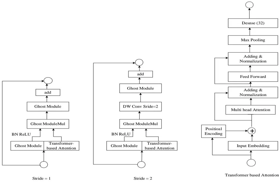
A model that can successfully extract minor information to distinguish between various materials is needed since XRD patterns can be noisy and complicated. The channel reduction and attention mechanisms of GhostNetV2 may be useful in this situation.
3.4.2. Bayesian Neural Network
The objective of classical learning is to identify a single optimal model parameter configuration, usually using maximum-likelihood optimization. As a result, the learner in the Bayesian framework observes the data and then infers a posterior distribution over the model's parameters . The posterior distribution is determined by Bayes rule, which is as follows: , where denotes prior distribution over parameters and is the likelihood of as determined by model with parameters . The Bayesian model average (BMA) is then used to determine the model's predictions for a fresh test sample .
Where, the predictive distribution for a specific value of the parameters w is denoted by . This BMA is especially persuasive in the context of Bayesian deep learning since, for a given issue, a contemporary neural network's posterior over parameters might reflect a multitude of complimentary solutions that correspond to various parameter values.
3.4.3. Feedforward Neural Network
FNN is one type of artificial neural network that is quite popular. Data moves through hidden layers of feedback-neutral network (FNN) in a single direction, from input layer to output layer. Numerous neurons make up each buried layer, which may be thought of as a linear change of the output from the layer before it. It is possible to characterize the basic functions of neurons as following equation (26).
Where, w stands for weight matrix, b is the bias vector, and X is the input vector.
A nonlinear processing of the neuron's output, controlled by activation function is necessary to increase the accuracy of network because many functions are linearly indivisible. The nonlinear transformation is then realized by converting the input, to a different value. For phase identification, sigmoid function is used as the activation function and it can be expressed as following equation (27).
The sigmoid function is frequently utilized in neural networks due to its stability and ease of derivation. A loss function is also necessary in order to assess the FNN's identification performance. In this FNN, cross-entropy function is selected as a loss function. A different loss function will be used to minimize the gradient since the sigmoid function's slope rapidly varies at both the upper and lower boundaries. The cross-entropy function may retain a high gradient because of its logarithmic nature, which is represented as following equation (28).
Where, denotes ideal output; represents actual output.
The mean is probably used to integrate results or predictions from the three models (BNN, FNN, and Improved GhostNetV2). The structure of mean is displayed in Fig. 4. The ensemble technique, which averages the predictions from several models, can yield a more reliable and accurate forecast. Mathematically this can be expressed in following equation (29).
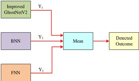
The mean reduces the biases and inaccuracies of individual models. This type of model averaging takes use of the variety of models that are used. The ensemble technique attempts to provide a more reliable and accurate overall forecast by integrating the strengths of each model, which may perform better in particular scenarios or with particular kinds of data.
III. RESULTS AND DISCUSSION
This section of this paper discusses about evaluation of results. The various metrics are taken for evaluate performance of proposed approach. The metrics are mainly used to analyse efficiency of suggested technique with various methods that are currently in use. The main objectives of this section are:
➢ Effectiveness of proposed technique using Sensitivity, Precision, Accuracy, Selectivity, FPR, NPV, F-score, MCC, and FNR;
➢ Comparison of the suggested approach with alternative existing techniques based on evaluation metrics.
The execution is performed in python platform.
4.1. Evaluation of metrics
The following metrics are used in the assessment of the proposed attack detection system:
Accuracy: It represents a percentage of total number of two correct guesses to total number of predictions in Eqn. (25).
Where, FP for False Positive, TP stands for True Positive, TN for True Negative, and FN for False Negative, an accuracy ratio of 1 denotes perfect accuracy, and 0 for a random guess.
Precision: It is defined as the ratio of the total amount of abnormal and normal data detected to the quantity of normal data detected, as given in Eqn. (26).
Sensitivity: It is defined as the ratio of total amount of data in dataset to number of normal data that were found, as shown in Eqn. (27).
F-score: The harmonic mean of precision and recall metrics is known as F-measure. It is represented in following Eqn. (28).
Specificity: The percentage of real negative cases that model properly detected is called Specificity, which is often referred to as True Negative Rate or Selectivity. Specificity is a binary classification performance measure. The formula for calculating specificity is as follows:
MCC: Matthews Correlation Coefficient or MCC is a statistic used to assess how well binary classification model is doing. The following Eqn. (30) is used to compute it:
NPV: A performance measure called Negative Predictive Value (NPV) is used in binary classification to assess how well a model predicts the negative class, or the occurrences that lack a specific condition or characteristic. The True Negative Rate is another name for NPV. The following Eqn. (31) is utilized to determine Negative Predictive Value:
FPR: The percentage of true negative occurrences that model mistakenly predicts as positive is called False Positive Rate (FPR), sometimes called False Alarm Rate. This performance statistic is utilized in binary classification. The below formula is used to compute it:
FNR: In binary classification, the False Negative Rate (FNR) is a performance indicator that quantifies the percentage of true positive occurrences that the model mistakenly predicts as negative. It is also known as the Miss Rate. The following formula is used to get FNR:
4.2. Evaluation of proposed technique with existing methods
The proposed technique is compared with various existing methods such as Improved GhostNetV2, BNN, and FNN to verify the performance of introduced strategy. For this purpose, the dataset is split for training and testing. Initially, the data is split as seventy percentage for training and thirty percent for testing. Further, the 80-percentage data was utilised for training purpose and the remaining data was used for testing. These split data was mainly used to ensure the effectiveness of developed method. The proposed and existing technique is analyzed with various evaluation metrics and these are discussed in following section. Table 1 depicts comparison result of proposed and existing method when data split is 70/30. The comparison between proposed and current methods when the data split is 80/20 is shown in Table 2.
| Model | Bayesian FusionNet | Improved GhostNetV2 | BNN | FNN |
| Accuracy | 0.98685 | 0.95054 | 0.93023 | 0.90909 |
| Precision | 0.98702 | 0.94148 | 0.92105 | 0.92105 |
| F-Score | 0.98385 | 0.94588 | 0.92105 | 0.85 |
| Specificity | 0.9878 | 0.94 | 0.94 | 0.94175 |
| Sensitivity | 0.98101 | 0.9775 | 0.90323 | 0.85714 |
| MCC | 0.98205 | 0.94118 | 0.90323 | 0.92683 |
| NPV | 0.98155 | 0.95161 | 0.92857 | 0.95223 |
| FPR | 0.04541 | 0.06341 | 0.05341 | 0.07341 |
| FNR | 0.03294 | 0.07954 | 0.06954 | 0.08954 |
| Model | Bayesian FusionNet | Improved GhostNetV2 | BNN | FNN |
| Accuracy | 0.99061 | 0.96591 | 0.94118 | 0.91023 |
| Precision | 0.98715 | 0.95588 | 0.9375 | 0.93878 |
| F-Score | 0.98719 | 0.95133 | 0.925 | 0.8534 |
| Specificity | 0.98281 | 0.94243 | 0.9434 | 0.9412 |
| Sensitivity | 0.98715 | 0.9612 | 0.93023 | 0.86364 |
| MCC | 0.989213 | 0.95082 | 0.92683 | 0.92563 |
| NPV | 0.989364 | 0.95455 | 0.93478 | 0.95238 |
| FPR | 0.03241 | 0.05341 | 0.03341 | 0.06341 |
| FNR | 0.02554 | 0.06954 | 0.04954 | 0.07954 |
The accuracy values of proposed, Improved GhostNetV2, BNN, and FNN are 0.98685, 0.95054, 0.93023, and 0.90909 respectively when 70 percentage data sets are involved for training and 30 percentage for testing. Similarly, when the data sets are split as 20 percentage for testing and 80 percentage for training, the accuracy values are denoted as 0.99061, 0.96591, 0.94118, and 0.91023 for proposed, Improved GhostNetV2, BNN, and FNN respectively. The aforementioned values states that the proposed method has highest accuracy than all other existing techniques. The graphical representation of accuracy analysis is shown in following Fig. 5.
{"image_source":{"path":"images/bdf4a7fd6dfdbb81885f3212ad82ebd43abd1d8bfdf4fd64e7172b871b78653e.jpg"},"content":"","chart_caption":[{"type":"text","content":"Figure 5: Analysis of accuracy"}],"chart_footnote":[]}
The suggested strategy, Improved GhostNetV2, BNN, and FNN have precision values of 0.98702, 0.94148, 0.92105, and 0.92105, respectively, when 70% of data sets are used for training and 30% are used for testing. Similar to this, precision scores for suggested method, Improved GhostNetV2, BNN, and FNN are stated as 0.98715, 0.95588, 0.9375, and 0.93878 correspondingly when the data sets are divided into 80 percent for training and 20 percent for testing. The results stated above indicate that the suggested method outperforms all other current methods in terms of precision. The following Fig. 6 displays precision analysis graphically.
{"image_source":{"path":"images/6758e535f8584e6ca4d57414868ad4d7dcb9f6f478bd0c0711008726c6f4e10b.jpg"},"content":"","chart_caption":[{"type":"text","content":"Figure 6: Analysis of precision"}],"chart_footnote":[]}
The F-score values of newly developed method, Improved GhostNetV2, FNN, and BNN are, respectively, 0.98385, 0.94588, 0.85, and 0.92105 with 70% of data sets are used for training and 30% for testing. Likewise, if data sets were divided into 80 percent for training and 20 percent for testing, the F-score results for suggested, BNN, Improved GhostNetV2, and FNN are stated as 0.98719, 0.925, 0.95133, and 0.8534 respectively. According to provided values, the suggested method is the most accurate F-score of all currently used methods. The F-score analysis is displayed graphically in Fig. 7 below.
{"image_source":{"path":"images/93543ab4c12210d1406ac70ee7948c7053070db1fb88d6a9009f46db8bc31eea.jpg"},"content":"","chart_caption":[{"type":"text","content":"Figure 7: Analysis of F-score"}],"chart_footnote":[]}
FNN, BNN, Improved GhostNetV2, and proposed approach have specificity values of 0.94175, 0.94, 0.94, and 0.9878 respectively, with 70% of the data sets utilized for testing and 30% for training. Similarly, if 80 percent of data sets are used to training and 20 percent are used for testing, specificity for FNN, BNN, Improved GhostNetV2 and, and proposed method are 0.9412, 0.9434, 0.94243, and 0.98281 respectively. The recommended approach has the highest specificity score among all presently employed methods, based on given information. Fig. 8 below shows a visual representation of the specificity analysis.
{"image_source":{"path":"images/b693852e947728cf07706e64e7f900aea250953f0f364978c4bc6124ebd7da0f.jpg"},"content":"","chart_caption":[{"type":"text","content":"Figure 8: Analysis of specificity"}],"chart_footnote":[]}
Improved GhostNetV2, FNN, BNN, and established strategy have sensitivity values of 0.9775, 0.85714, 0.90323, and 0.98101 respectively, with 70% of the data sets employed for testing and 30% for too.0oraining. Similarly, the sensitivity for recommended, BNN, Improved GhostNetV2, and FNN are 0.980....715, 0.93023, 0.9612, and 0.86364 respectively, if the data sets are split into 80 percentage for training and 20% for testing. The recommended approach has the highest sensitivity among all presently employed methods, based on aforementioned results. Figure 9 below shows a visual representation of the sensitivity analysis.
{"image_source":{"path":"images/5b6bcf81743d3c0a23ecb2b4f7aba655fcb05600ee0440dbbe89350b87aebb25.jpg"},"content":"","chart_caption":[{"type":"text","content":"Figure 9: Analysis of sensitivity"}],"chart_footnote":[]}
The MCC values are listed as 0.98205 for proposed technique, 0.94118 for Improved GhostNetV2, 0.92683 for FNN, and 0.90323 for BNN with 70% of data sets utilized for training and 30 percentage for testing. Similarly, if data sets are split 80 percent for training and 20 percent for testing, the MCC values are 0.989213 for recommended approach, 0.92683 for BNN, 0.95082 for Improved GhostNetV2, and 0.92563 for FNN. Based on information provided above, the proposed approach has the highest MCC value among all presently available methods. Fig. 10 below shows an illustration of MCC evaluation.
{"image_source":{"path":"images/0219975381b1e1481959b34135187cc1bc90f5f3993f4b979bd5b95e2ef4f483.jpg"},"content":"","chart_caption":[{"type":"text","content":"Figure 10: Analysis of MCC"}],"chart_footnote":[]}
The NPV values for 70% of data sets used for training and 30% for testing are 0.98155 for proposed approach, 0.95161 for Improved GhostNetV2, 0.95223 for FNN, and 0.92857 for BNN. Similar to this, the NPV values for recommended technique is 0.989364, 0.93478 for BNN, 0.95455 for Improved GhostNetV2, and 0.95238 for FNN if the data sets are divided 80 percent for training and 20 percent for testing. Out of all currently accessible approaches, the suggested strategy has the greatest NPV value according to information presented above. Figure 11 below provides an example of NPV evaluation.
{"image_source":{"path":"images/0de9c08079f2277a1050f9248b0e1f4fc24278d4939f5d64ce6fe63c25b74728.jpg"},"content":"","chart_caption":[{"type":"text","content":"Figure 11: Analysis of NPV"}],"chart_footnote":[]} When 70% of data sets are utilized for training and 30% are used for testing, the FPR values of proposed approach, FNN, BNN, and Improved GhostNetV2 are 0.04541, 0.07341, 0.05341, and 0.06341, respectively. Similarly, with the data sets split 80 percent for training and 20 percent for testing, the accuracy scores for the proposed technique, BNN, Improved GhostNetV2, and FNN are 0.03241, 0.03341, 0.05341, and 0.06341, respectively. The above-mentioned results show that the recommended method performs more precisely than any other existing method. The subsequent Fig. 12 illustrates FPR analysis visually.
{"image_source":{"path":"images/8210da6df36fcc726673c57e30b763dc86830e71e6ad8585c1b3ac9dc4b92bbf.jpg"},"content":"","chart_caption":[{"type":"text","content":"Figure 12: Analysis of FPR"}],"chart_footnote":[]}
The methods FNN, Improved GhostNetV2, BNN, and the recommended strategy have FNR values of 0.08954, 0.07954, 0.06954, and 0.03294, respectively, when 70% of data sets are utilized for training and 30% for testing. Similar to this, when the data sets are split into 80 percent for training and 20 percent for testing, FNR scores for recommended technique, BNN, Improved GhostNetV2, and FNN are reported as 0.02554, 0.04954, 0.06954, and 0.07954 accordingly. The aforementioned findings show that recommended strategy performs more precisely than any other existing approach in terms of FNR. The following Fig.13 is visually displayed the evaluation of FNR.
{"image_source":{"path":"images/b7de62cc95f106c5c359dd464e781474be0cd08abaebb224c4e57c4639c4ca54.jpg"},"content":"","chart_caption":[{"type":"text","content":"Figure 13: Analysis of FNR"}],"chart_footnote":[]} From above evaluation results, the suggested approach exceeds current techniques in a range of assessment measures. The suggested method outperforms Improved GhostNetV2, BNN, and FNN in terms of accuracy, precision, F-score, specificity, sensitivity, MCC, NPV, and reduced FPR when trained with 70% of the data. Even with 80% more training data, this pattern continues. Its solid performance across numerous assessment criteria is demonstrated by superiority of suggested technique in terms of F-score, accuracy, precision, sensitivity, specificity, MCC, reduced FPR, and NPV.
IV. CONCLUSION
This study presents a novel framework using a hybridized machine learning technique for autonomous phase detection in X-ray diffraction. The procedure includes a rigorous pre-processing step that includes data cleaning, normalization, and smoothing. This is followed by a multi-pronged feature extraction step that extracts important information such as peak position, intensity, and statistical characteristics. HWSKO, a novel hybrid optimization technique, is used to choose features, which successfully lowers computational complexity and improves model performance. Compared to previous techniques, the Bayesian FusionNet-based phase identification shows superiority across several assessment measures by integrating Improved GhostNetV2, Bayesian Neural Network, and Feedforward Neural Network. The outcomes demonstrate that the suggested method is successful even with a larger training dataset in terms of accuracy, precision, and other important parameters. This extensive framework highlights the promise of a hybridized machine learning technique for furthering material science research and enabling effective analysis across a range of applications, in addition to automating phase detection in X-ray diffraction.
Future studies might investigate the incorporation of increasingly more sophisticated designs to improve the Bayesian FusionNet as neural network technology advances. Further research into attention processes, recurrent neural networks, or innovative convolutional neural networks (CNNs) may improve the model's capacity to identify complex patterns in XRD data. An important step forward would be to improve the suggested technique for real-time applications. The process entails enhancing the Bayesian FusionNet computing performance to facilitate swift phase identification, hence making it suitable for real-time analysis in material science labs or industrial environments.
ABSTRACT
The Dja Biosphere Reserve is home to immense natural resources. Increasing poaching and other human activities like shifting cultivation and industrial agriculture are major problems in this area. This study addresses the need to explore the attitude and perception of local residents toward wildlife and conservation. Questionnaires, surveys and field observations were used in data collection. A total of 400 people was conveniently selected in 16 villages from October to December 2015. Data analysis relied mainly on factor analysis and structural equation modelling in SPSS 21 and Smart-PLS software. The main findings indicate a significant positive relationship between wildlife education, community wildlife sensitization and the local attitude on community involvement in conservation, which in turn have a strong and positive significant impact on the perception of the local people towards wildlife and conservation. Moreover, the perception of local people has a significant positive impact on the level of discipline towards wildlife and conservation.
Language: English
Conflict of Interest
The authors declare no conflict of interest.
Ethical Approval
Not applicable
Data Availability
The datasets used in this study are openly available at [repository link] and the source code is available on GitHub at [GitHub link].
Funding
This work did not receive any external funding.
References
Cite this article
Related Research


Special Issue
Launch a focused special issue to highlight research, emerging trends, and expert insights in your academic field.