Prony Analysis -A Case Study in Eastern Regional Power System in India

# I. INTRODUCTION Day by day, the power system is becoming increasingly complex due to the growing demand for electricity and the widespread integration of power electronic devices. As a result, the power grid is undergoing continuous and rapid changes. These developments introduce several operational challenges and contingencies, making timely monitoring of system data crucial for identifying faults and preventing major economic losses [1-3]. 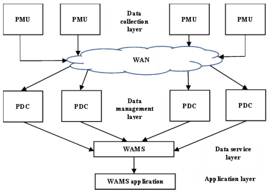Traditionally, utilities have relied on Remote Terminal Units (RTUs) in Supervisory Control and Data Acquisition (SCADA) systems, which provide system information to operators every 4 to 10 seconds. However, this steady-state data is no longer sufficient for effective monitoring, control, and operation of large interconnected grids [4,5]. To overcome these limitations, a more advanced technology—synchronized measurement technology—has been introduced, and systems based on this concept are known as Wide Area Measurement Systems (WAMS). The key device in synchronized measurement technology is the Phasor Measurement Unit (PMU). A PMU is generally defined as a device that measures the magnitude, phase angle, frequency, and rate of change of frequency of electrical quantities in real time. These measurements are synchronized with GPS signals. The overall process from data collection to WAMS applications is shown in Fig. 1 [6]. At the substation, the PMU receives both analog and digital inputs, filters them using an anti-aliasing filter, converts analog data into digital form, and performs phasor estimation. The phasor data is then transmitted through a modem. IEEE Standard C37.118-2011 specifies the measurement requirements, communication message formats, and protection classes for PMU data. The GPS-synchronized PMU data is transmitted to a Phasor Data Concentrator (PDC) through various communication channels. The PDC collects, sorts, and time-aligns the data based on timestamps and measurement types. Using communication networks, this processed data is then forwarded to SCADA or WAMS control centres. Finally, the data supports a wide range of WAMS applications, including real-time monitoring, control, protection, and post-event (historian) analysis [6].  In this paper, Section 2 describes the TEESTA-III case study, Prony analysis, and its implementation in MATLAB. Section 3 presents the results obtained from the Prony analysis, and Section 4 provides the conclusions drawn from the analyses performed. # II. PRONY ANALYSIS The Prony method was introduced by Gaspard de Prony, a French engineer, mathematician, and scientist. Prony analysis is an extension of the Fast Fourier Transform (FFT), and it fits a linear combination of damped exponential terms to a uniformly sampled signal. The general linear exponential function is defined as given in equation (1) [9-13]. The estimation of low-frequency inter-area oscillations is challenging when using a conventional SCADA system, as its measurements are derived from RTUs. RTUs cannot provide synchronized phasor measurements of voltage, current, and system frequency at multiple locations with the same time stamp. Therefore, for transient and dynamic analysis, the required data must be obtained from Phasor Measurement Units (PMUs), which provide time-synchronized measurements essential for accurate oscillation analysis. $$ X (t) = \sum_ {i = 1} ^ {P} A _ {i} e ^ {\alpha i t} \cos \left(\omega_ {i} t + \theta_ {i}\right) \tag {1} $$ Where $i = 1$ to $P$ (number of damping exponential modes), $A_i$ is the amplitude, $\alpha_i$ is the damping factor, $\omega_i$ is the frequency, and $\theta_i$ is the phase angle. Prony analysis gives a complete analysis of the given signal by providing amplitude, phase, frequency, and damping coefficients of the signal, whereas Fourier analysis does not provide the damping coefficients. After applying Euler's formula and after approximations, the above formula is deduced to the following function, $$ X (t) = \sum_ {i = 1} ^ {P} \frac {1}{2} A _ {i} \left(e ^ {j \Theta_ {i}} e ^ {\lambda^ {+} t} + e ^ {- j \Theta_ {i}} e ^ {\lambda^ {-} t}\right) \tag {2} $$ Where, $\lambda = \sigma_{\mathrm{i}} \pm \mathrm{j}\omega_{i}$ , are the eigen values of the system. The above equation can also be written as follows $$ \mathrm {X} (\mathrm {t}) = \sum_ {\mathrm {i} = 1} ^ {\mathrm {P}} \mathrm {B} _ {\mathrm {i}} \mathrm {e} ^ {\lambda \mathrm {i t}} \tag {3} $$ Let the above is sampled at intervals of time period 'T', then the above equation for $\mathrm{X(t)}$ can be expressed as, $$ \mathrm {X} (\mathrm {t}) = \sum_ {\mathrm {i} = 1} ^ {\mathrm {P}} \mathrm {B} _ {\mathrm {i}} \mathrm {e} ^ {\lambda \mathrm {i t}} \tag {4} $$ $$ \mathrm {X} (\mathrm {t}) = \sum_ {\mathrm {i} = 1} ^ {\mathrm {P}} \mathrm {B} _ {\mathrm {i}} \mathrm {e} ^ {\lambda \mathrm {i k T}} = \sum_ {\mathrm {i} = 1} ^ {\mathrm {P}} \mathrm {B} _ {\mathrm {i}} \mu_ {i} ^ {\mathrm {k}} \tag {5} $$ Where, $\mathrm{k} = 0,1,2,\ldots$ N-1; $\mathrm{N} =$ total number of samples From the above equations it is clear that if we find out the values of $\mathrm{B}$ and $\mu$ we can get the values of $\mathrm{A}$ and $\alpha$ , which will decide the presence of oscillations. The following method is used in Prony analysis to find the values of $\mathrm{B}$ and $\mu$ . $$ \left[ \begin{array}{c} \mathrm {X} (0) \\ \mathrm {X} (1) \\ \vdots \\ \mathrm {X} (\mathrm {N} - 1) \end{array} \right] = \left[ \begin{array}{c c c c} 1 & 1 & \dots & 1 \\ \mu_ {1} & \mu_ {2} & \dots & \mu_ {\mathrm {m}} \\ \vdots & \vdots & & \vdots \\ \mu_ {1} ^ {\mathrm {N} - 1} & \mu_ {2} ^ {\mathrm {N} - 1} & \dots & \mu_ {\mathrm {m}} ^ {\mathrm {N} - 1} \end{array} \right] \left[ \begin{array}{c} \mathrm {B} _ {1} \\ \mathrm {B} _ {2} \\ \vdots \\ \mathrm {B} _ {\mathrm {m}} \end{array} \right] \tag {6} $$ In generalized form the above matrix can be written as follows, $$ [ X ] = [ U ] [ b ] \tag {7} $$ The M values of $\mu$ , can be considered as a solution of the following polynomial with $\alpha_{i}$ as unknown coefficients, $$ \mu^ {\mathrm {m}} - \mathrm {a} _ {1} \mu^ {\mathrm {m} - 1} - \mathrm {a} _ {1} \mu^ {\mathrm {m} - 2} \dots \dots \dots \dots \dots - \mathrm {a} _ {\mathrm {m}} = 0 \tag {8} $$ the 'a' can be represented in the vector form as follows, $$ \hat {a} = \left[ - a _ {m}, - a _ {m - 1}, \dots, - a _ {1}, 1, 0, \dots, 0 \right] \tag {9} $$ on multiplying the (6) and (9) equations we get $$ \hat {a} X = X (m) - \left[ - a _ {m} X (0) - a _ {m - 1} X (1) \dots \dots - a _ {1} X (m - 1) \right] = \hat {a} [ U ] [ b ] \tag {10} $$ $$ = B _ {1} \left[ \mu_ {1} ^ {\mathrm {m}} - \left(a _ {1} \mu^ {\mathrm {m} - 1} - a _ {\mathrm {m}} \mu_ {1} ^ {\mathrm {m} - 1} + \dots . + a _ {\mathrm {m}} \mu_ {1} ^ {0}\right) \right] + B _ {2} [ \dots . ] + \dots . = 0 \tag {11} $$ The initial time instant is assumed, then the above equation is written as, $$ \left[ \begin{array}{c} \mathrm {X} (\mathrm {m}) \\ \mathrm {X} (\mathrm {m} + 1) \\ \vdots \\ \mathrm {X} (\mathrm {N} - 1) \end{array} \right] = \left[ \begin{array}{c c c} \mathrm {X} (\mathrm {m} + 1) \dots & \mathrm {X} (0) \\ \mathrm {X} (\mathrm {m}) & \dots & \mathrm {X} (1) \\ \vdots & & \vdots \\ \mathrm {X} (\mathrm {N} - 2) & \dots & \mathrm {X} (\mathrm {N} - \mathrm {m} - 1) \end{array} \right] \left[ \begin{array}{c} a _ {1} \\ a _ {2} \\ \vdots \\ a _ {\mathrm {m}} \end{array} \right] \tag {12} $$ The above matrix can be written as, $$ [ \mathrm {d} ] = [ \mathrm {D} ] [ \mathrm {a} ] \tag {13} $$ Assume $N > 2m$ , the coefficient vector 'a' is calculated as, $$ [ \mathrm {a} ] = [ \mathrm {D} ^ {\prime} ] [ \mathrm {d} ] \tag {14} $$ $D$ is pseudo inverse of $\mathrm{d}$ After we find vector 'a', the $\mu$ can be easily found out and finally we can find out B, and after that we can easily get the amplitude 'A' and damping factor 'a'. Prony analysis can be performed on various discrete signals of power, voltage, current, and frequency. In this project, the frequencies are taken into consideration and we can perform modal analysis. Prony analysis is basically a measurement-based analysis, which does not require any network model of the system. Using the real-time data obtained from the eastern region of the Indian power system, Prony analysis has been performed and the respective frequency components, damping, and amplitudes are found. This analysis helps in finding out the dominant low-frequency components in the system; thereby, we can estimate the low-frequency oscillations in the system [9-13]. The theoretical superiority of Prony analysis for this study lies in its resolution and damping extraction capabilities. FFT suffers from spectral leakage when analysing short, transient data windows and cannot distinguish between two closely spaced modes if the record length is insufficient. Prony analysis, being a parametric technique, is not limited by the uncertainty principle of the Fourier transform, allowing it to resolve low-frequency inter-area modes (0.1-0.8 Hz) even from short post-fault data records. Furthermore, the ability to directly quantify negative or low damping provides actionable data for the tuning of Power System Stabilizers (PSS), which FFT magnitude plots cannot provide. # 2.1 Case Study in Eastern Region of India - TEESTA-III Event Description On $07^{\mathrm{th}}$ of July 2017, at 10:26:00 hrs, a $400\mathrm{kV}$ Rangpo-Binaguri (RB)-II line tripped due to a line-to-ground fault in phase-B, which caused congestion in the $400\mathrm{kV}$ RB-I line. This is mitigated by the System Protection Scheme (SPS)-I at Teesta-III by tripping generating units at Chujachen (at 0.84 s), JLHEP, and Dikchu (both at 1.70 s) power stations. However, the RB-I line remained congested and caused the tripping of the $400\mathrm{kV}$ Teesta-III-Rangpo (at 2.50 s) single-circuit line (loss of 400 MW load). This is followed by the tripping of remaining units at Teesta-III and Dikchu (at 3.00 s) due to loss of evacuation path. The PMU data of this event is collected from 12 PMUs at different locations in the eastern region of India, as shown in Figure 3, to perform the Prony analysis. The different locations are Bihar, Binaguri, Durgapur, Farakka, Jeypore, Patna, Ranchi, Rourkela, Sasaram, Talcher, Relangi, and Jamshedpur.  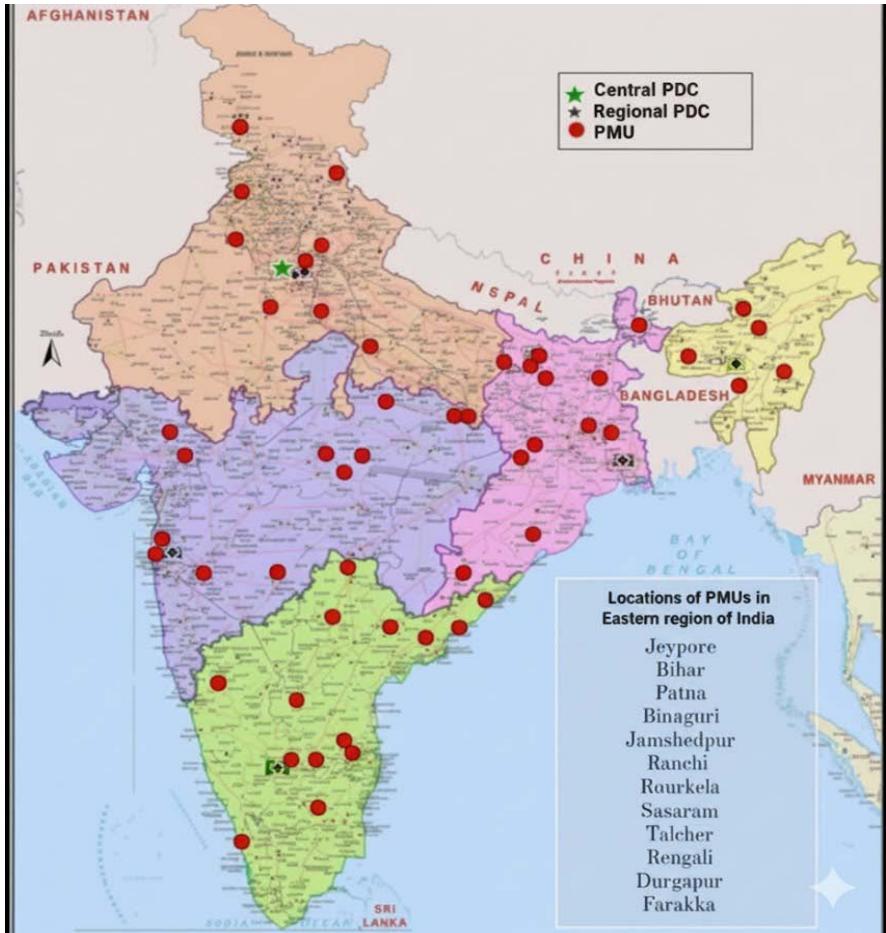Fig. 2: Locations of PMUs in India During the TEESTA-III Event on $07^{\text{th}}$ July 2017 # 2.2 Prony Analysis on TEESTA-III Data The real-time historian data has been provided by the Eastern Region Power Grid, and it has been obtained from PMUs at 12 different locations, namely Bihar, Binaguri, Durgapur, Farakka, Jeypore, Patna, Ranchi, Rourkela, Sasaram, Talcher, Relangi, and Jamshedpur, along with the time stamps. In Prony analysis, the actual frequency variation with time is first plotted. The obtained signal is then detrended, as detrending improves the accuracy of the analysis. After detrending, the Prony fit for each signal is obtained, and the Prony-approximated linear curves for different locations are shown in Figures (3-14). The sampling frequency of the obtained data from the Eastern Region Power Grid is $25\mathrm{Hz}$ . Hence, for satisfactory Prony analysis, the model order (M) must be at least half of the number of samples (N), i.e., 12.5. Therefore, the model order is chosen as 13 in this case [10].  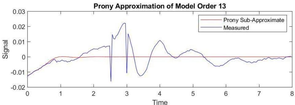Fig. 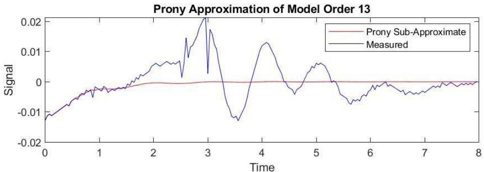3: Frequency Variation after Detrending and Prony Fit at Bihar  Fig. 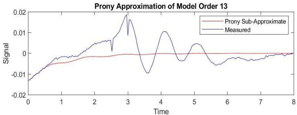4: Frequency Variation after Detrending and Prony Fit at Durgapur  Fig. 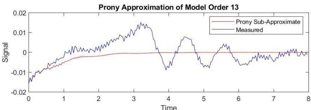5: Frequency Variation after Detrending and Prony Fit at Farakka  Fig. 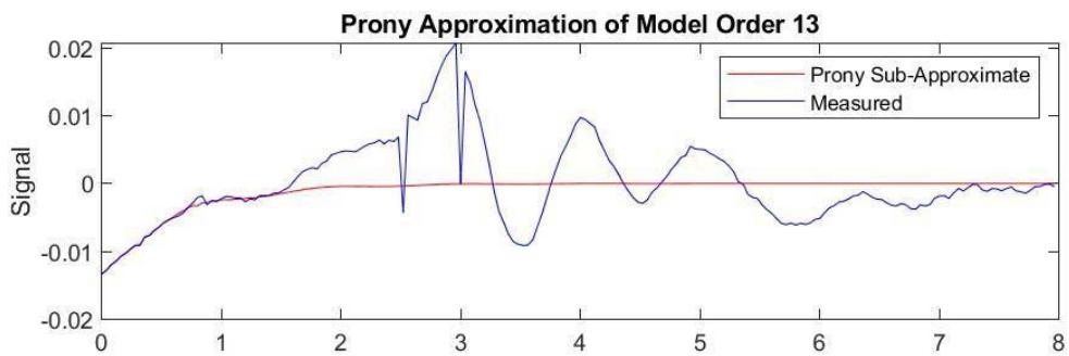6: Frequency Variation after Detrending and Prony Fit at Jeypore  Fig. 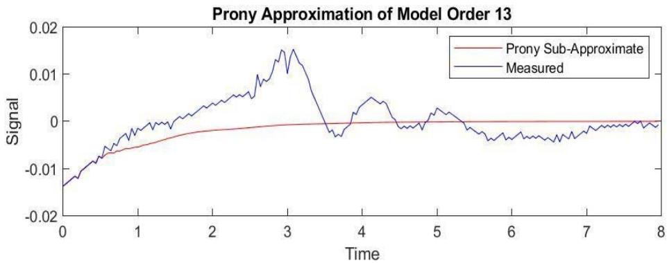7: Frequency Variation after Detrending and Prony fit at Patna  Fig. 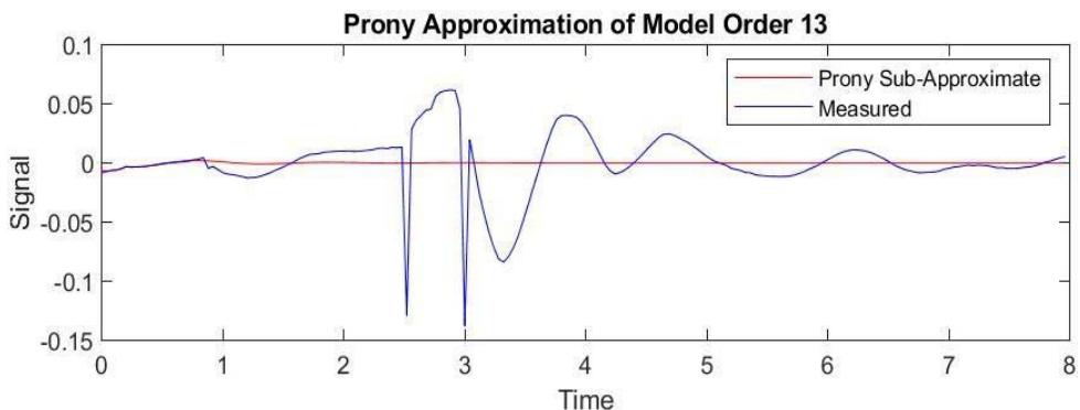8: Frequency Variation after Detrending and Prony Fit at Ranchi  Fig. 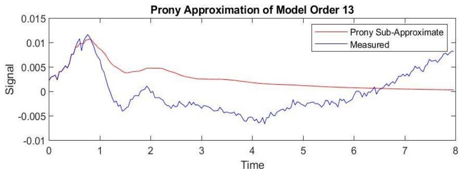9: Frequency Variation and Prony Fit at Binaguri  Fig. 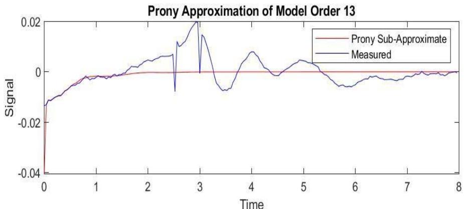10: Frequency Variation after Detrending and Prony Fit at Rourkela  Fig. 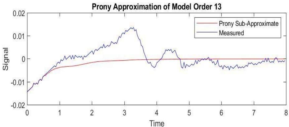11: Frequency variation after detrending and Prony fit at Sasaram  Fig. 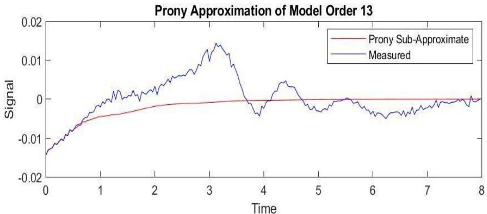12: Frequency variation after detrending and Prony fit at Talcher  Fig. 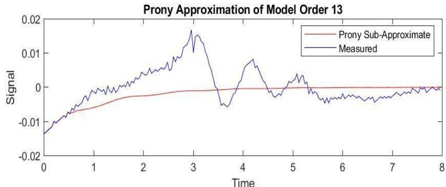13: Frequency Variation after Detrending and Prony Fit at Rengali  Fig. 14: Frequency Variation after Detrending and Prony Fit at Jamshedpur # III. RESULTS # 3.1 Prony Analysis on Eastern Region of India Prony analysis is performed on the Indian Eastern Grid data, and the respective frequency components present at different locations are tabulated. The mean squared error (MSE) between the original signal and the Prony fit is also calculated and presented in the figures. Table 1: Prony Analysis of Frequency Variation at Bihar <table><tr><td>Mode</td><td>Amplitude(Hz)</td><td>Damping(%)</td><td>Frequency(Hz)</td><td>Energy(J)</td></tr><tr><td>1</td><td>3.9e-02</td><td>3.4</td><td>0.031</td><td>1.6e-03</td></tr><tr><td>2</td><td>5.3e-03</td><td>1.9</td><td>0.9</td><td>5.0e-05</td></tr><tr><td>3</td><td>5.3e-03</td><td>1.9</td><td>0.9</td><td>5.0e-05</td></tr> <tr><td>4</td><td>2.6e-04</td><td>1.4</td><td>10</td><td>1.6e-09</td></tr><tr><td>5</td><td>2.6e-04</td><td>1.4</td><td>10</td><td>1.6e-09</td></tr><tr><td>6</td><td>1.6e-04</td><td>1.5</td><td>8.3</td><td>5.7e-09</td></tr><tr><td>7</td><td>1.6e-04</td><td>1.5</td><td>8.3</td><td>5.7e-09</td></tr><tr><td>8</td><td>1.5e-04</td><td>1.9</td><td>3.9</td><td>4.0e-09</td></tr><tr><td>9</td><td>1.5e-04</td><td>1.9</td><td>3.9</td><td>4.0e-08</td></tr><tr><td>10</td><td>0.92e-04</td><td>1.4</td><td>12</td><td>2.0e-09</td></tr><tr><td>11</td><td>1.7e-05</td><td>1.7</td><td>6.2</td><td>5.8e-10</td></tr><tr><td>12</td><td>1.7e-05</td><td>1.7</td><td>6.2</td><td>5.8e-10</td></tr></table>  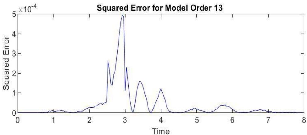Fig. 15: Mean squared error of Prony analysis at Bihar Table 1 shows the respective modes of frequencies, damping, energies, and their corresponding amplitudes at Bihar. Generally, frequencies between $0 - 2\mathrm{Hz}$ can be considered as electromechanical oscillations. From the results, it can be seen that the oscillations with frequencies $0.0031\mathrm{Hz}$ and $0.9\mathrm{Hz}$ are treated as low-frequency oscillations, and their damping is less than $10\%$ ; therefore, they may cause small-signal instability. As Prony analysis cannot differentiate noise signals, those with energy greater than $10^{-5}$ are considered spurious signals. Figure 15 shows the mean squared error between the original signal and the Prony approximation at Bihar. Table 2: Prony Analysis of Frequency Variation at Binaguri <table><tr><td>Mode</td><td>Amplitude (Hz)</td><td>Damping (%)</td><td>Frequency (Hz)</td><td>Energy (J)</td></tr><tr><td>1</td><td>1.1e-02</td><td>1.1</td><td>1.8</td><td>5.1e-03</td></tr><tr><td>2</td><td>1.1e-02</td><td>1.1</td><td>1.81</td><td>5.1e-05</td></tr><tr><td>3</td><td>5.5e-03</td><td>1.3</td><td>0.92</td><td>7.8e-05</td></tr><tr><td>4</td><td>5.5e-03</td><td>1.3</td><td>0.92</td><td>7.8e-05</td></tr><tr><td>5</td><td>4.4e-04</td><td>2.2</td><td>4.1</td><td>3.0e-07</td></tr><tr><td>6</td><td>4.4e-04</td><td>2.2</td><td>4.1</td><td>3.0e-07</td></tr><tr><td>7</td><td>3.3e-04</td><td>1.6</td><td>6.3</td><td>2.2e-09</td></tr><tr><td>8</td><td>3.3e-04</td><td>1.6</td><td>6.31</td><td>2.2e-09</td></tr><tr><td>9</td><td>2.6e-04</td><td>1.5</td><td>8.4</td><td>1.5e-08</td></tr><tr><td>10</td><td>2.6e-04</td><td>1.5</td><td>8.4</td><td>1.5e-09</td></tr><tr><td>11</td><td>1.9e-04</td><td>1.3</td><td>10</td><td>9.2e-08</td></tr><tr><td>12</td><td>1.9e-04</td><td>1.3</td><td>10</td><td>9.2e-08</td></tr></table>  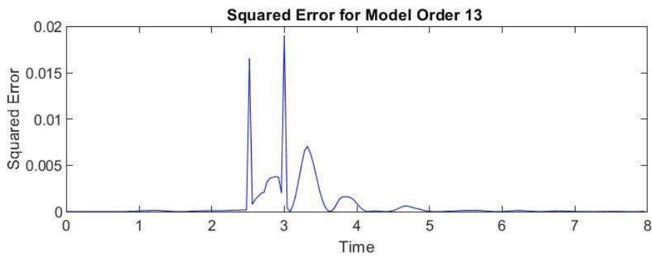Fig. 16: Mean Squared Error of Prony Analysis at Binaguri Table 2 shows the respective modes, frequencies, damping, energies, and their corresponding amplitudes at Binaguri. From the results, it can be seen that the oscillations with frequencies 1.8, 1.81, and $0.92\mathrm{Hz}$ are treated as low-frequency oscillations. Their energy is below the threshold, and their damping is less than $10\%$ , so they may cause small-signal instability. As Prony analysis cannot differentiate noise signals, signals with energy greater than $10^{-5}$ are considered spurious. Figure 16 shows the mean squared error between the original signal and the Prony approximation at Binaguri. Table 3: Prony analysis of frequency variation at Durgapur <table><tr><td>Mode</td><td>Amplitude (Hz)</td><td>Damping (%)</td><td>Frequency (Hz)</td><td>Energy (J)</td></tr><tr><td>1</td><td>2.4e-02</td><td>0.97</td><td>0.03</td><td>1.9e-03</td></tr><tr><td>2</td><td>9.6e-04</td><td>0.45</td><td>0.9</td><td>6.4e-05</td></tr><tr><td>3</td><td>9.6e-04</td><td>1.45</td><td>0.9</td><td>6.4e-05</td></tr><tr><td>4</td><td>3.9e-04</td><td>1.7</td><td>10</td><td>3.0e-07</td></tr><tr><td>5</td><td>3.9e-04</td><td>1.7</td><td>10</td><td>3.0e-07</td></tr><tr><td>6</td><td>2.7e-04</td><td>1.6</td><td>12</td><td>1.5e-07</td></tr><tr><td>7</td><td>2.4e-04</td><td>1.9</td><td>4</td><td>1.0e-07</td></tr><tr><td>8</td><td>2.4e-04</td><td>1.9</td><td>4</td><td>1.0e-07</td></tr><tr><td>9</td><td>1.4e-04</td><td>1.9</td><td>6.2</td><td>3.7e-08</td></tr><tr><td>10</td><td>1.4e-04</td><td>1.9</td><td>6.2</td><td>3.8e-08</td></tr><tr><td>11</td><td>9.4e-05</td><td>1.7</td><td>8.3</td><td>1.8e-08</td></tr><tr><td>12</td><td>9.4e-05</td><td>1.7</td><td>8.3</td><td>1.8e-08</td></tr></table>  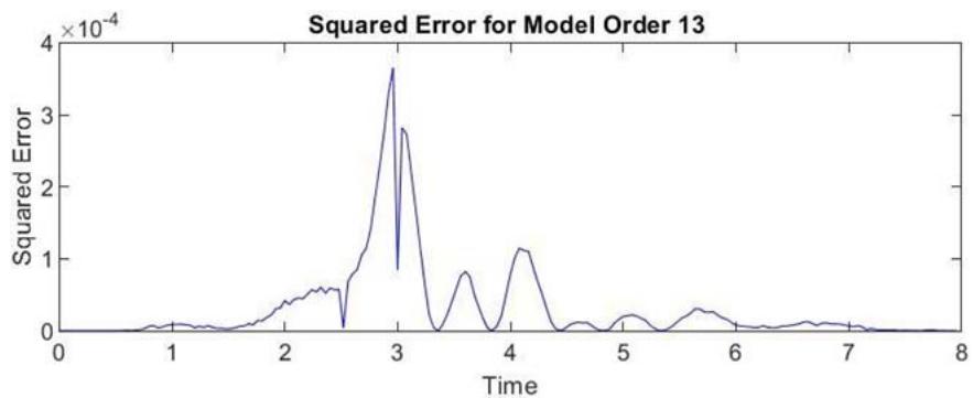Fig. 17: Mean squared error of Prony analysis at Durgapur Table 3 shows the respective modes, frequencies, damping, energies, and their corresponding amplitudes at Durgapur. From the results, it can be seen that the oscillations with frequencies 0.03 and $0.9\mathrm{Hz}$ are treated as low-frequency oscillations. Their energy is below the threshold, and their damping is less than $10\%$ , so they may cause small-signal instability. As Prony analysis cannot differentiate noise signals, the signals with energy greater than $10^{-5}$ are considered spurious. Figure 17 shows the mean squared error between the original signal and the Prony approximation at Durgapur. Table 4: Prony Analysis of Frequency Variation at Farakka <table><tr><td>Mode</td><td>Amplitude(Hz)</td><td>Damping(%)</td><td>Frequency(Hz)</td><td>Energy(J)</td></tr><tr><td>1</td><td>2.4e-02</td><td>1.4</td><td>0.03</td><td>1.4e-03</td></tr><tr><td>2</td><td>1.3e-02</td><td>39</td><td>12</td><td>4.5e-05</td></tr><tr><td>3</td><td>1.2e-02</td><td>18</td><td>12</td><td>4.6e-05</td></tr><tr><td>4</td><td>1.2e-03</td><td>6.4</td><td>0.89</td><td>7.7e-05</td></tr><tr><td>5</td><td>1.2e-03</td><td>6.4</td><td>0.89</td><td>7.7e-05</td></tr><tr><td>6</td><td>8.8e-04</td><td>3.2</td><td>11</td><td>8.6e-07</td></tr><tr><td>7</td><td>8.8e-04</td><td>3.2</td><td>11</td><td>8.6e-07</td></tr><tr><td>8</td><td>5.0e-04</td><td>2.0</td><td>3.9</td><td>4.3e-07</td></tr><tr><td>9</td><td>5.0e-04</td><td>2.0</td><td>3.9</td><td>4.3e-07</td></tr><tr><td>10</td><td>4.4e-04</td><td>1.9</td><td>6.2</td><td>3.6e-07</td></tr><tr><td>11</td><td>4.5e-04</td><td>1.9</td><td>6.2</td><td>3.6e-07</td></tr><tr><td>12</td><td>4.4e-04</td><td>2.0</td><td>8.6</td><td>3.3e-07</td></tr><tr><td>13</td><td>4.4e-04</td><td>2.0</td><td>8.6</td><td>3.3e-07</td></tr></table>  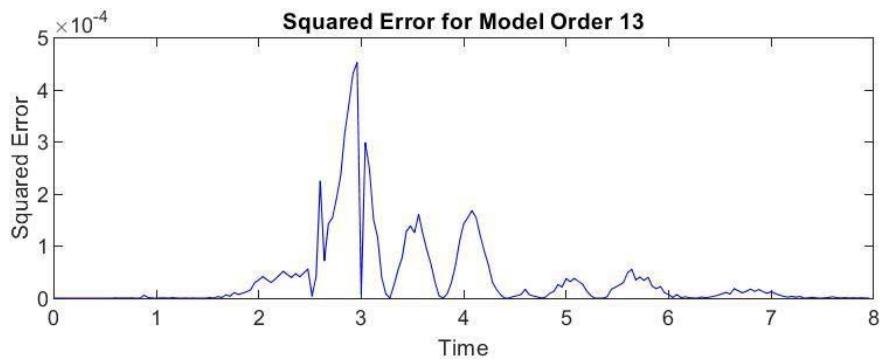Fig. 18: Mean Squared Error of Prony Analysis at Farakka Table 4 shows the respective modes, frequencies, damping, energies, and their corresponding amplitudes at Farakka. From the results, it can be seen that the oscillations with frequencies 0.03 and $0.89\mathrm{Hz}$ are treated as low-frequency oscillations, which decay very slowly, and their energy is below the threshold. Their damping is also less than $10\%$ , so they may cause small-signal instability. The $12\mathrm{Hz}$ component is likely noise, as it is damped out very fast with damping values of $39\%$ and $18\%$ . As Prony analysis cannot differentiate noise signals, signals with energy greater than $10^{-5}$ are considered spurious. Figure 18 shows the mean squared error between the original signal and the Prony approximation at Farakka. Table 5: Prony Analysis of Frequency Variation at Patna <table><tr><td>Mode</td><td>Amplitude(Hz)</td><td>Damping(%)</td><td>Frequency(Hz)</td><td>Energy(J)</td></tr><tr><td>1</td><td>2.6e-02</td><td>1.5</td><td>0.03</td><td>1.4e-03</td></tr><tr><td>2</td><td>1.3e-03</td><td>0.98</td><td>0.91</td><td>5.5e-06</td></tr><tr><td>3</td><td>1.3e-03</td><td>0.98</td><td>0.91</td><td>5.5e-06</td></tr><tr><td>4</td><td>2.6e-04</td><td>1.8</td><td>12</td><td>1.3e-07</td></tr><tr><td>5</td><td>2.4e-04</td><td>1.7</td><td>10</td><td>1.2e-07</td></tr><tr><td>6</td><td>2.4e-04</td><td>1.7</td><td>10</td><td>1.2e-07</td></tr><tr><td>7</td><td>1.8e-04</td><td>1.7</td><td>8.3</td><td>6.9e-08</td></tr><tr><td>8</td><td>1.8e-04</td><td>1.7</td><td>8.3</td><td>6.9e-08</td></tr><tr><td>9</td><td>1.5e-04</td><td>1.8</td><td>3.9</td><td>4.0e-08</td></tr><tr><td>10</td><td>1.5e-04</td><td>1.8</td><td>3.9</td><td>4.0e-08</td></tr><tr><td>11</td><td>1.2e-04</td><td>1.9</td><td>6.2</td><td>2.8e-08</td></tr><tr><td>12</td><td>1.2e-04</td><td>1.9</td><td>6.2</td><td>2.8e-08</td></tr></table>  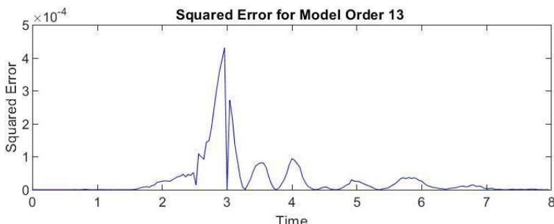Fig. 19: Mean Squared Error of Prony Analysis at Patna Table 5 shows the respective modes, frequencies, damping, energies, and their corresponding amplitudes at Patna. From the results, it can be seen that the oscillations with frequencies 0.03 and $0.91\mathrm{Hz}$ are treated as low-frequency oscillations. Their energy is below the threshold, and their damping is also less than $10\%$ , so they may cause small-signal instability. As Prony analysis cannot differentiate noise signals, signals with energy greater than $10^{-5}$ are considered spurious. Figure 19 shows the mean squared error between the original signal and the Prony approximation at Patna. Table 6: Prony Analysis of Frequency Variation at Jeypore <table><tr><td>Mode</td><td>Amplitude(Hz)</td><td>Damping(%)</td><td>Frequency(Hz)</td><td>Energy(J)</td></tr><tr><td>1</td><td>3.0e-02</td><td>1.2</td><td>0.03</td><td>2.6e-03</td></tr><tr><td>2</td><td>3.4e-03</td><td>13</td><td>6.1</td><td>4.4e-06</td></tr><tr><td>3</td><td>1.3e-03</td><td>0.69</td><td>0.84</td><td>8.0e-05</td></tr><tr><td>4</td><td>1.3e-03</td><td>0.69</td><td>0.84</td><td>8.0e-05</td></tr><tr><td>5</td><td>1.2e-03</td><td>2.4</td><td>3.8</td><td>2e-06</td></tr><tr><td>6</td><td>1.2e-03</td><td>2.4</td><td>3.8</td><td>2e-06</td></tr><tr><td>7</td><td>1.2e-03</td><td>2.9</td><td>6.8</td><td>1.7e-06</td></tr><tr><td>8</td><td>1.2e-03</td><td>2.9</td><td>6.8</td><td>1.7e-06</td></tr><tr><td>9</td><td>8.5e-04</td><td>0.9</td><td>12.1</td><td>2.6e-06</td></tr><tr><td>10</td><td>8.5e-04</td><td>0.9</td><td>12</td><td>2.6e-06</td></tr><tr><td>11</td><td>3.5e-04</td><td>2.4</td><td>9.3</td><td>1.8e-07</td></tr><tr><td>12</td><td>3.5e-04</td><td>2.4</td><td>9.3</td><td>1.8e-07</td></tr></table>  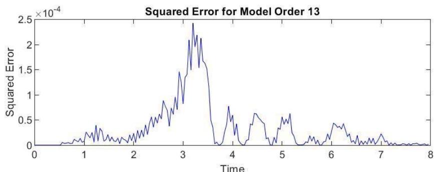Fig. 20: Mean squared error of Prony analysis at Jeypore Table 6 shows the respective modes, frequencies, damping, energies, and their corresponding amplitudes at Jeypore. From the results, it can be seen that the oscillations with frequencies 0.03 and $0.84\mathrm{Hz}$ are treated as low-frequency oscillations. Their energy is below the threshold, and their damping is also less than $10\%$ , so they may cause small-signal instability. The 6.1 Hz component is likely noise, as it is damped out very fast with a damping of $13\%$ . As Prony analysis cannot differentiate noise signals, signals with energy greater than $10^{-5}$ are considered spurious. Figure 20 shows the mean squared error between the original signal and the Prony approximation at Jeypore. Table 7: Prony Analysis of Frequency Variation at Ranchi <table><tr><td>Mode</td><td>Amplitude(Hz)</td><td>Damping(%)</td><td>Frequency(Hz)</td><td>Energy(J)</td></tr><tr><td>1</td><td>4.4e-02</td><td>22</td><td>11</td><td>5.9e-05</td></tr><tr><td>2</td><td>4.4e-02</td><td>22</td><td>11</td><td>5.9e-05</td></tr><tr><td>3</td><td>2.7e-02</td><td>0.94</td><td>0.031</td><td>2.4e-03</td></tr><tr><td>4</td><td>7.7e-03</td><td>6.9</td><td>12</td><td>3.5e-05</td></tr><tr><td>5</td><td>7.7e-03</td><td>6.9</td><td>12</td><td>3.5e-05</td></tr><tr><td>6</td><td>1.2e-03</td><td>2.8</td><td>8.6</td><td>1.8e-06</td></tr><tr><td>7</td><td>1.2e-03</td><td>2.8</td><td>8.6</td><td>1.8e-06</td></tr><tr><td>8</td><td>1.1e-03</td><td>1.0</td><td>8.1</td><td>3.6e-06</td></tr><tr><td>9</td><td>1.1e-03</td><td>1.0</td><td>8.1</td><td>3.6e-06</td></tr><tr><td>10</td><td>4.0e-04</td><td>2.2</td><td>3.9</td><td>2.4e-07</td></tr><tr><td>11</td><td>4.0e-04</td><td>2.2</td><td>3.9</td><td>2.4e-07</td></tr><tr><td>12</td><td>3.5e-04</td><td>3.3</td><td>6.3</td><td>1.3e-07</td></tr><tr><td>13</td><td>3.5e-04</td><td>3.3</td><td>6.3</td><td>1.3e-07</td></tr></table>  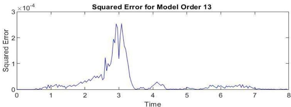Fig. 21: Mean Squared Error of Prony Analysis at Ranchi Table 7 shows the respective modes, frequencies, damping, energies, and their corresponding amplitudes at Ranchi. From the results, it can be seen that the oscillation with frequency $0.031\mathrm{Hz}$ is treated as a low-frequency oscillation. Its energy is below the threshold, and its damping is also less than $10\%$ , so it may cause small-signal instability. The $11\mathrm{Hz}$ component is likely noise, as it is damped out very fast with a damping of $22\%$ . As Prony analysis cannot differentiate noise signals, signals with energy greater than $10^{-5}$ are considered spurious. Figure 21 shows the mean squared error between the original signal and the Prony approximation at Ranchi. Table 8: Prony Analysis of Frequency Variation at Rourkela <table><tr><td>Mode</td><td>Amplitude(Hz)</td><td>Damping(%)</td><td>Frequency(Hz)</td><td>Energy(J)</td></tr><tr><td>1</td><td>2.1e-02</td><td>0.43</td><td>0.031</td><td>3.2e-03</td></tr><tr><td>2</td><td>7.7e-03</td><td>1.1</td><td>0.73</td><td>1.8e-04</td></tr><tr><td>3</td><td>7.7e-03</td><td>1.1</td><td>0.73</td><td>1.8e-04</td></tr><tr><td>4</td><td>4.6e-03</td><td>7.3</td><td>12</td><td>1.2e-06</td></tr><tr><td>5</td><td>4.6e-03</td><td>7.3</td><td>12</td><td>1.2e-06</td></tr><tr><td>6</td><td>1.5e-03</td><td>3.1</td><td>10</td><td>2.5e-06</td></tr> <tr><td>7</td><td>1.5e-03</td><td>3.1</td><td>10</td><td>2.5e-06</td></tr><tr><td>8</td><td>8.8e-04</td><td>4.1</td><td>7.5</td><td>6.9e-07</td></tr><tr><td>9</td><td>8.8e-04</td><td>4.1</td><td>7.5</td><td>6.9e-07</td></tr><tr><td>10</td><td>8.0e-04</td><td>4.0</td><td>5.9</td><td>5.8e-07</td></tr><tr><td>11</td><td>8.0e-04</td><td>4.0</td><td>5.9</td><td>5.8e-07</td></tr><tr><td>12</td><td>6.8e-04</td><td>1.1</td><td>3.5</td><td>1.3e-06</td></tr><tr><td>13</td><td>6.8e-04</td><td>1.1</td><td>3.5</td><td>1.3e-06</td></tr></table>  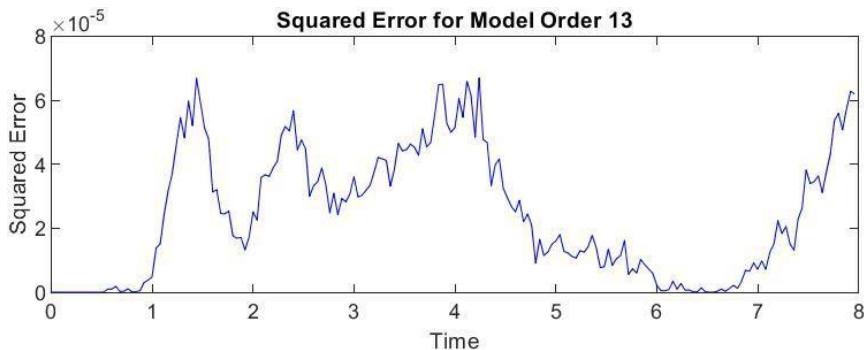Fig. 22: Mean Squared Error of Prony Analysis at Rourkela Table 8 shows the respective modes, frequencies, damping, energies, and their corresponding amplitudes at Rourkela. From the results, it can be seen that the oscillations with frequencies 0.03 and $0.73\mathrm{Hz}$ are treated as low-frequency oscillations. Their energy is below the threshold, and their damping is also less than $10\%$ , so they may cause small-signal instability. As Prony analysis cannot differentiate noise signals, signals with energy greater than $10^{-5}$ are considered spurious. Figure 22 shows the mean squared error between the original signal and the Prony approximation at Rourkela. Table 9: Prony Analysis of Frequency Variation at Sasaram <table><tr><td>Mode</td><td>Amplitude(Hz)</td><td>Damping(%)</td><td>Frequency(Hz)</td><td>Energy(J)</td></tr><tr><td>1</td><td>5.8e-02</td><td>68</td><td>0.03</td><td>8.4e-05</td></tr><tr><td>2</td><td>2.4e-02</td><td>1.7</td><td>0.031</td><td>1.2e-03</td></tr><tr><td>3</td><td>3.0e-03</td><td>1.5</td><td>0.91</td><td>2.0e-05</td></tr><tr><td>4</td><td>3.0e-03</td><td>1.5</td><td>0.91</td><td>2.0e-05</td></tr><tr><td>5</td><td>3.6e-04</td><td>1.7</td><td>6.2</td><td>2.5e-07</td></tr><tr><td>6</td><td>3.6e-04</td><td>1.7</td><td>6.2</td><td>2.5e-07</td></tr><tr><td>7</td><td>2.6e-04</td><td>1.6</td><td>3.9</td><td>1.4e-07</td></tr><tr><td>8</td><td>2.6e-04</td><td>1.6</td><td>3.9</td><td>1.4e-07</td></tr><tr><td>9</td><td>1.7e-04</td><td>1.7</td><td>8.3</td><td>5.6e-08</td></tr><tr><td>10</td><td>1.7e-04</td><td>1.7</td><td>8.3</td><td>5.6e-08</td></tr><tr><td>11</td><td>1.2e-04</td><td>1.6</td><td>10</td><td>3.2e-08</td></tr><tr><td>12</td><td>1.2e-04</td><td>1.6</td><td>11</td><td>3.2e-08</td></tr></table>  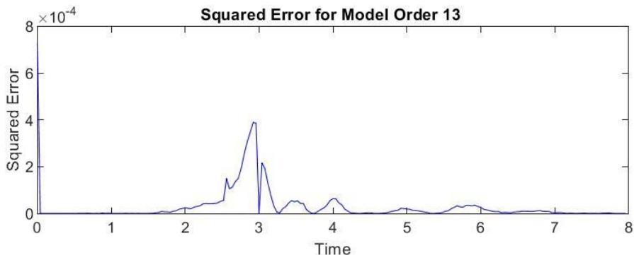Fig. 23: Mean squared error of Prony analysis at Sasaram Table 9 shows the respective modes, frequencies, damping, energies, and their corresponding amplitudes at Sasaram. From the results, it can be seen that the oscillations with frequencies 0.03 and $0.91\mathrm{Hz}$ are treated as low-frequency oscillations. Their energy is below the threshold, and their damping is also less than $10\%$ , so they may cause small-signal instability. As Prony analysis cannot differentiate noise signals, signals with energy greater than $10^{-5}$ are considered spurious. Figure 23 shows the mean squared error between the original signal and the Prony approximation at Sasaram. Table 10: Prony Analysis of Frequency Variation at Talcher <table><tr><td>Mode</td><td>Amplitude(Hz)</td><td>Damping(%)</td><td>Frequency(Hz)</td><td>Energy(J)</td></tr><tr><td>1</td><td>2.4e-02</td><td>1.0</td><td>0.031</td><td>1.9e-05</td></tr><tr><td>2</td><td>4.0e-03</td><td>6.2</td><td>8.0</td><td>1.0e-06</td></tr><tr><td>3</td><td>4.0e-03</td><td>6.2</td><td>8.0</td><td>1.0e-06</td></tr><tr><td>4</td><td>2.9e-03</td><td>5.7</td><td>9.4</td><td>6.0e-06</td></tr><tr><td>5</td><td>2.9e-03</td><td>5.7</td><td>9.4</td><td>6.0e-06</td></tr><tr><td>6</td><td>2.5e-03</td><td>5.7</td><td>6.0</td><td>4.2e-06</td></tr><tr><td>7</td><td>2.5e-03</td><td>5.7</td><td>6.0</td><td>4.2e-06</td></tr><tr><td>8</td><td>2.3e-03</td><td>1.3</td><td>0.75</td><td>1.4e-05</td></tr><tr><td>9</td><td>2.3e-03</td><td>1.3</td><td>0.75</td><td>1.4e-05</td></tr><tr><td>10</td><td>5.5e-04</td><td>3.0</td><td>3.6</td><td>3.5e-07</td></tr><tr><td>11</td><td>5.5e-04</td><td>3.0</td><td>3.6</td><td>3.5e-07</td></tr><tr><td>12</td><td>5.4e-04</td><td>3.9</td><td>11</td><td>2.8e-07</td></tr><tr><td>13</td><td>5.4e-04</td><td>3.9</td><td>11</td><td>2.8e-07</td></tr></table>  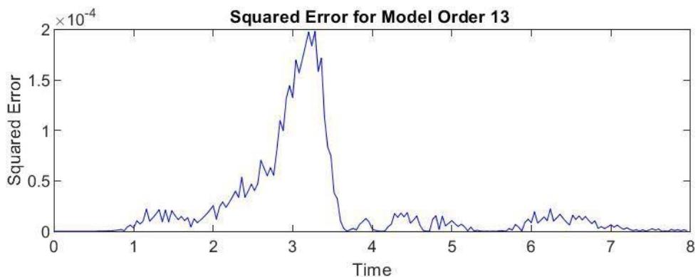Fig. 24: Mean Squared Error of Prony Analysis at Talcher Table 10 shows the respective modes, frequencies, damping, energies, and their corresponding amplitudes at Talcher. From the results, it can be seen that the oscillation with frequency $0.031\mathrm{Hz}$ is treated as a low-frequency oscillation. Its energy is below the threshold, and its damping is also less than $10\%$ , so it may cause small-signal instability. As Prony analysis cannot differentiate noise signals, signals with energy greater than $10^{-5}$ are considered spurious. Figure 24 shows the mean squared error between the original signal and the Prony approximation at Talcher. Table 11: Prony Analysis of Frequency Variation at Rengali <table><tr><td>Mode</td><td>Amplitude(Hz)</td><td>Damping(%)</td><td>Frequency(Hz)</td><td>Energy(J)</td></tr><tr><td>1</td><td>2.5e-02</td><td>0.93</td><td>0.031</td><td>2.2e-03</td></tr><tr><td>2</td><td>1.3e-03</td><td>0.94</td><td>0.71</td><td>6.2e-03</td></tr><tr><td>3</td><td>1.3e-03</td><td>0.94</td><td>0.71</td><td>6.2e-03</td></tr><tr><td>4</td><td>1.1e-03</td><td>2.8</td><td>1.2</td><td>1.6e-04</td></tr><tr><td>5</td><td>1.1e-03</td><td>2.8</td><td>1.2</td><td>1.6e-04</td></tr><tr><td>6</td><td>7.0e-04</td><td>5.6</td><td>5.8</td><td>3.4e-07</td></tr><tr><td>7</td><td>7.0e-04</td><td>5.6</td><td>5.8</td><td>3.4e-07</td></tr><tr><td>8</td><td>6.2e-04</td><td>2.3</td><td>9.5</td><td>5.7e-07</td></tr><tr><td>9</td><td>6.2e-04</td><td>2.3</td><td>9.5</td><td>5.7e-07</td></tr><tr><td>10</td><td>4.2e-04</td><td>3.3</td><td>7.4</td><td>2.0e-07</td></tr><tr><td>11</td><td>4.2e-04</td><td>3.3</td><td>7.4</td><td>2.0e-07</td></tr><tr><td>12</td><td>4.2e-04</td><td>2.3</td><td>3.7</td><td>2.4e-07</td></tr><tr><td>13</td><td>4.2e-04</td><td>2.3</td><td>3.7</td><td>2.4e-07</td></tr></table>  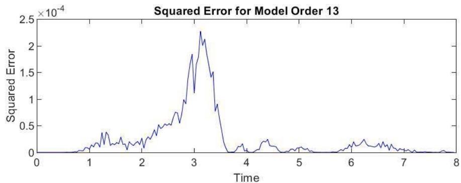Fig. 25: Mean Squared Error of Prony Analysis at Rengali Table 11 shows the respective modes, frequencies, damping, energies, and their corresponding amplitudes at Rengali. From the results, it can be seen that the oscillations with frequencies 0.031, 1.2, and $0.71\mathrm{Hz}$ are treated as low-frequency oscillations. Their energy is below the threshold, and their damping is also less than $10\%$ , so they may cause small-signal instability. As Prony analysis cannot differentiate noise signals, signals with energy greater than $10^{-5}$ are considered spurious. Figure 25 shows the mean squared error between the original signal and the Prony approximation at Rengali. Table 12: Prony analysis of frequency variation at Jamshedpur <table><tr><td>Mode</td><td>Amplitude(Hz)</td><td>Damping(%)</td><td>Frequency(Hz)</td><td>Energy(J)</td></tr><tr><td>1</td><td>3.8e-02</td><td>13</td><td>12</td><td>5.6e-04</td></tr><tr><td>2</td><td>2.5e-02</td><td>0.83</td><td>0.031</td><td>2.5e-03</td></tr><tr><td>3</td><td>1.3e-02</td><td>8.0</td><td>11</td><td>1.0e-07</td></tr><tr><td>4</td><td>1.3e-02</td><td>8.0</td><td>11</td><td>6.0e-07</td></tr><tr><td>5</td><td>9.3e-04</td><td>3.8</td><td>8.3</td><td>6.0e-07</td></tr><tr><td>6</td><td>9.3e-04</td><td>3.8</td><td>8.3</td><td>4.2e-07</td></tr><tr><td>7</td><td>9.1e-04</td><td>3.6</td><td>6.3</td><td>4.2e-07</td></tr><tr><td>8</td><td>9.1e-04</td><td>3.6</td><td>6.3</td><td>1.4e-07</td></tr> <tr><td>9</td><td>8.0e-04</td><td>5.7</td><td>0.87</td><td>3.5e-05</td></tr><tr><td>10</td><td>8.0e-04</td><td>5.7</td><td>0.87</td><td>3.5e-05</td></tr><tr><td>11</td><td>3.6e-04</td><td>3.7</td><td>4.0</td><td>1.2e-07</td></tr><tr><td>12</td><td>3.6e-04</td><td>3.7</td><td>4.0</td><td>1.2e-07</td></tr></table>  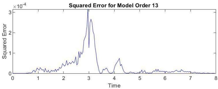Fig. 26: Mean Squared Error of Prony Analysis at Jamshedpur Table 12 shows the respective modes, frequencies, damping, energies, and their corresponding amplitudes at Jamshedpur. From the results, it can be seen that the oscillations with frequencies 0.031 and $0.87\mathrm{Hz}$ are treated as low-frequency oscillations. Their energy is below the threshold, and their damping is also less than $10\%$ , so they may cause small-signal instability. The $12\mathrm{Hz}$ component is likely noise, as it is damped out very fast with a damping of $13\%$ . As Prony analysis cannot differentiate noise signals, signals with energy greater than $10^{-5}$ are considered spurious. Figure 26 shows the mean squared error between the original signal and the Prony approximation at Jamshedpur. # IV. CONCLUSION The stability of the Indian Eastern Regional Grid is frequently compromised by poorly damped Low-Frequency Oscillations (LFOs), a vulnerability amplified during system transients. This paper presents a detailed modal analysis of the cascading event that occurred on July 7, 2017, initiated by a fault on the $400\mathrm{kV}$ Rangpo-Binaguri (RB)-II line, which led to the System Protection Scheme (SPS) action and the eventual loss of the Teesta-III corridor. High-resolution synchrophasor data from 12 Phasor Measurement Units (PMUs) across the region were processed using Prony Analysis to accurately extract the frequency, damping percentage, and energy of the oscillatory modes. The low-frequency oscillations (LFOs) were detected at various locations. It was found that the $0.031\mathrm{Hz}$ component of LFOs is present at almost all locations, with comparatively low damping, indicating that this component requires close monitoring to prevent potential small-signal instability. At Binaguri and Rengali, most of the LFOs were observed, with frequencies of 1.8, 1.81, $0.92\mathrm{Hz}$ and 0.031, 0.71, $1.2\mathrm{Hz}$ respectively. Although the amplitudes of these LFOs are low at all locations, the damping is consistently below $10\%$ , indicating that the LFOs are somewhat predominant and sustain for a longer duration, which may cause small-signal instability in the system. Spurious noise signals were also observed at all locations, highlighting the inability of Prony analysis to differentiate between actual and noise signals. The mean squared error across all locations confirms the high accuracy of the Prony analysis. For performing these analyses, the data obtained from PMUs is the fundamental building block. It can be concluded that for real-time dynamic monitoring and obtaining accurate results, WAMS plays a critical role. Hence, a Wide Area Measurement System (WAMS) enhances the operation, monitoring, and control of complex power systems through synchrophasor measurement technology.

Generating HTML Viewer...