




IntelliPaper
Abstract
International regulatory organizations for quality control of X-ray systems, such as the International Atomic Energy Agency (IAEA), have implemented protocols for acceptance
testing of digital mammography and breast tomosyn thesis equipment, aiming to establish quality standards in radiology services. However, these guidelines are usually based on tests with breast phantoms with standardized thicknesses and compositions, often not representative of the patient population profiles at those services. In a prior study, we developed a computational system designed to automatically tracking and managing data extracted from the image acquisition processes of digital mammography and breast tomosyn thesis, stored on a DICOM SCP (Service Class Provider) server. This approach enables obtaining technical reports characterizing exposure parameters and tests have shown that the reference levels outlined in international standards for breast composition and radiation dose do not accurately reflect the characteristics of the actual patient population. Thus this study describes data collection and corresponding analysis for the dose tracking process primarily on three digital mammography systems of different radiological services. Extensive image datasets from these systems were obtained using a new application described previously, with a focus on dose profiles generated during exposures. Graphical representations resulting from the datasets are presented, along with analysis of skin entrance and mean glandular doses distributions, average kV and mAs applied during the exams together with the target/filter combinations, radiographic density distributions, as well as the age and breast thickness characteristic of the respective population submitted to exposures in each of those mammography services. Additionally, the extent of information and ease of acquisition provided by the tool for performance evaluation of digital mammography services is discussed.
Explore Digital Article Text
I. INTRODUCTION
Breast cancer, according to World Health Organization [1], accounts for an estimated 2.3 million new cases, as reported in 2020. The same estimation indicates probably about 15.5 million cases in 2030. The highest mortality rate due to breast cancer in Brazil, for instance, is observed in the Southeast region, with 16.14 deaths per 100,000 women. This highlights the importance not only of self-examination but also of undergoing examinations such as mammography. Furthermore, it is crucial to adhere to quality and safety standards when conducting such examinations regarding the benefit of patients.
In order to ensure comprehensive breast imaging while optimizing the number of images and minimizing the radiation exposure to the patient, two main projections are employed in mammography: mediolateral-oblique (MLO) and craniocaudal (CC) [2]. This approach also reduces the areas not exposed to the X-ray beam, which is captured on the imaging plane.
Optimal generation of the X-ray beam is crucially important, aligning with the chosen imaging acquisition method, meaning that photons should have energy within the optimal range. As the selection of the anode/filter material of the X-ray tube varies according to its performance for certain breast thicknesses and density, the material selection can be relevant to acquire the best image quality with the lowest radiation dose for the patient.
The application of diagnosis standards is decisive to ensure the quality of radiological services, as emphasized in the IEC 61223-1 standard [3]. This standard not only covers the quality aspects of mammography equipment but also covers operational techniques and acceptance tests. Furthermore, guidelines for digital mammography quality have been developed, taking into account test results, particularly those obtained using phantoms defined in national and international standards. These guidelines primarily focus on standard breast thicknesses and glandular composition, although it is well known that breast composition can vary among different populations [4-6].
Consequently, determining the characteristic features of each specific population is important in order to establish reference levels for radiation doses absorbed by breast tissue. In current digital mammography procedures, all images are recorded in accordance with the DICOM (Digital Imaging and Communication in Medicine) protocol , which includes essential information about the examination and exposure conditions, such as breast thickness and the dose received by the breast during the procedure, among other information. Therefore, investigating this technical data from the DICOM header can contribute to enhancing the image acquisition process.
By properly using anode/filter combination, in addition to the electrical parameters of the equipment, the Skin Entrance Dose (SED) and the Mean Glandular Dose (MGD) can be minimized. These values can be measured and associated with patient images through the DICOM protocol.
Therefore, the development of a computational tool that uses data extracted from these files to provide information on dose profiles could effectively manage the image acquisition process. This tool, in conjunction with the characterization of the population profile, could complement the standard quality assurance tests in digital mammography. By following the quality criteria required by medical professionals and international standards, this approach aims to improve the overall quality of digital mammography examinations.
Our team previously conducted a study aiming to extract relevant data from DICOM headers of a collection of 2D digital mammography and digital breast tomosynthesis images. Modifications to this previous approach, developed in JAVA language, resulted in software tested using a database consisting of mammography cases from patients exposed to a FFDM (Full Field Digital Mammography) equipment at a public hospital in Brazil . In such a study , the responses of the DICOM header from a set of images were evaluated and compared with quality control tests conducted in practice. The purpose was to estimate the actual mean glandular dose (MGD) using a calibrated dosimeter (Accu-Gold AGMS-M +, Radcal, Monrovia, CA) based on the values of kerma measured with PMMA and those calculated for the breast tissue in a digital mammography system. The calculation of MGD was based on Dance's method , which involved the product of some parameters such as air kerma, standard density, standard thickness, half-value layer (HVL), and the target-filter combination.
Once validated the effectiveness of our software (named ReadDICOM) through that investigation [9], the current study focuses on the evaluation of many correlations possible to extract from the data contained in DICOM headers regarding the mammography images from the exams performed in FFDM equipment. Here not only aspects of patient doses based on breast thickness or age are considered, but also the parameters of the X-ray equipment used as well as aspects on radiographic density. The purpose is to provide a comprehensive temporal analysis of examination procedures in a mammography service, focusing on dosimetry aspects and their relationship with the population characteristics of the patients undergoing these examinations.
II. METHODS AND MATERIALS
The images used for analysis were obtained at 3 radiological facilities installed in public hospitals in the state of Sao Paulo, Brazil. All of those radiological services used GE FFDM (Senographe DS or Senographe Essential) mammography equipment at the time the examinations corresponding to the present study were conducted. From the "Radiological Unit 1", our database stored information from mammography examinations of 380 patients (exams between November and December, 2013); from the "Unit 2", in turn, data was collected from examinations of 63 patients (exams between October, 2013 and February, 2015), while from "Unit 3" the total recorded data referred to examinations conducted on 1,025 patients (in this last case, about 5,000 exposures – images). However, this last dataset was divided into smaller sets to facilitate the analysis. Therefore, for this current description, a set of 1,367 images, representing exams of almost 300 patients (performed between June 2016 and June 2019) was taken into account for the main statistics.
One of the essential tools for conducting the study was the ReadDICOM software , developed in JavaScript, which is responsible for extracting the DICOM header data from each image file and organizing this information into a spreadsheet file. The user-friendly interface of the program allowed for easy extraction of all the necessary information for subsequent analyses in less than one minute for each images set. Once the data spreadsheet was complete, data pre-processing was performed. Initially, patients with a high number of missing data were excluded from the study as they were deemed irrelevant. Additionally, the acquisition date attribute and patient age were standardized.
After completing the data pre-processing, the following study profiles were defined for correlation analysis, similar to : (a) patient identification, mammography machine, and examination date; (b) type of breast projection; (c) Voltage and, current-time parameter, and anode/filter materials; (d) breast thickness and compression force; (d) Skin Entrance Dose (SED) and Mean Glandular Dose (MGD) values.
In the population profile, we evaluated general patients aspects for the purpose of establishing correlations with the mammographic exam. The graphical analyses conducted are detailed below:
1. Distribution of cases based on patients breasts thickness;
2. Distribution of patients based on their ages;
3. Distribution of average breast thickness among patients according to their identified age;
4. Distribution of cases by thickness - separated by images projection: CC and MLO;
- Histogram illustrating the distribution of cases divided into breast thickness ranges.
These analyses allowed for mapping the most relevant characteristics of the population served by those radiological services. For the dosimetry profile, which constitutes the primary focus of this study, the objective was to conduct quantitative and qualitative evaluations of the radiation doses received by the patients. The following relations were generated:
-
Histogram of Skin Entrance Dose (SED) values based on breast thickness ranges – by projection (CC and MLO) and overall;
-
Histogram of Mean Glandular Dose (MGD) values based on breast thickness ranges – by projection (CC and MLO) and overall;
-
Histogram illustrating the distribution of MGD in terms of the total number of exposures based on dose value ranges;
4. Average SED based on patient ages within the dataset;
5. Average MGD based on patient ages within the dataset;
6. Average SED and MGD received by patients;
- Percentage of cases above the mean and standard deviation of SED and MGD per breast thickness range;
8. Histogram of the number of images taken for each target/filter combination;
- Distribution of the number of patients per average breast thickness range, considering all images taken in a single examination.
These correlations provided fundamental insights into the behavior of the mammography equipment and its determination of radiation doses in each exposure.
Lastly, for the creation of the operational profile, operational parameter data (kVp and mAs) recorded during the mammographic exposures, in conjunction with the used target/filter combinations, were considered. The following graphical correlations were generated:
- Average kVp and mAs values per breast thickness range during the examinations for the respective tube target/filter combinations: (a) Rh/Rh; (b) Mo/Rh; (c) Mo/Mo;
2. Average kVp and mAs values for all target/filter combinations;
- Percentage of cases for the used target/filter combinations.
These correlations provided insights into the operational aspects of the mammography equipment, including the selection of target/filter combinations and the associated parameter values.
Furthermore, data were determined on the sizes of breast areas relative to all the images as well as their radiographic density. This was provided by using the latest version of the LIBRA software (Breast Imaging Group, UPenn) [11] on all image sets obtained from the 3 digital mammography units. As a result, this approach allowed determining an outcome corresponding to the profile of each set in terms of density variation (within the BIRADS ranges).
III. RESULTS
From the analysis of the image sets described in the previous section, we have determined initially the population profile of patients undergoing examinations on those mammography units during the respective time periods considered in the beginning of section 2. The results are graphically illustrated in Fig. 1, 2 and 3.
{"image_source":{"path":"images/8bb0491e486781efaf6ecf2fa6a0074d6a41ca3cbef7400b00565a2f59494cbe.jpg"},"content":"","chart_caption":[{"type":"text","content":"Number of patients/thicknesses"},{"type":"text","content":"(a)"}],"chart_footnote":[]} {"image_source":{"path":"images/4eed108042a2ca9dc819261e8b56bbd693eb028ba681992695dafb1b553fdeaf.jpg"},"content":"","chart_caption":[{"type":"text","content":"Number of patients by age"},{"type":"text","content":"(b)"}],"chart_footnote":[]}
{"image_source":{"path":"images/500e48b233d5445cb0655177c268754699e701d3f77f36043c6c4cf46419ee92.jpg"},"content":"","chart_caption":[{"type":"text","content":"Number of patients/thicknesses (overview: 1000 patients)"},{"type":"text","content":"(c)"},{"type":"text","content":"Fig. 1: Population Histogram I: Distribution of Cases According to Patients' Breast Thickness (a) for UNIT 1; (b) for UNIT 2 and (c) for UNIT 3"}],"chart_footnote":[]} {"image_source":{"path":"images/0e2e672137bab997b0561560017e79665e9bfff2f1dfeb54fda861c11abeb57a.jpg"},"content":"","chart_caption":[{"type":"text","content":"Number of patients per age"},{"type":"text","content":"(a)"},{"type":"text","content":"Radiation Dose Tracking in Digital Mammography: Evaluation of Population Profiles through Automatic Data Extraction from the DICOM Header"}],"chart_footnote":[]}
{"image_source":{"path":"images/ff30820059b6b9edf134ab203a1babc46f78ec3a18826fb66b76f8a923191da1.jpg"},"content":"","chart_caption":[{"type":"text","content":"Number of patients/thicknesses"},{"type":"text","content":"(b)"}],"chart_footnote":[]} {"image_source":{"path":"images/8dec57594e963cda39219e0e322263d49254bb1f9f297f2bd37370cd5fa1dd6e.jpg"},"content":"","chart_caption":[{"type":"text","content":"Number of patients/thicknesses (overview: 1000 patients)"},{"type":"text","content":"(c)"},{"type":"text","content":"Fig. 2: Population Histogram II: Distribution of Cases According to Patient age (a) for UNIT 1; (b) for UNIT 2 and (c) for UNIT 3"}],"chart_footnote":[]}
{"image_source":{"path":"images/f8ea36252b8ecca1c1ee50ab173e05168bee4346533f905ee02d4b483a74a971.jpg"},"content":"","chart_caption":[{"type":"text","content":"Total of cases per thickness range"},{"type":"text","content":"(a)"}],"chart_footnote":[]} {"image_source":{"path":"images/241ff87b49af1e4db5536f35d2e1e3efa3fe897cad1d3dceeedb22c2f104cde8.jpg"},"content":"","chart_caption":[{"type":"text","content":"Number of cases by thickness ranges"}],"chart_footnote":[]}
{"image_source":{"path":"images/e0860634c5d37231eeb5a79d1e977684365cd78dd9747aa0cc640b0e57c61567.jpg"},"content":"","chart_caption":[{"type":"text","content":"(b)"},{"type":"text","content":"(c)"},{"type":"text","content":"Fig. 3: Histogram of Case Distribution by Thickness Separated by Breast Thickness Ranges. (a) for UNIT 1; (b) for UNIT 2 and (c) for UNIT 3"}],"chart_footnote":[]}
Organizations such as EUREF (European Reference Organization for Quality Assured Breast Screening and Diagnostic Services) use PMMA simulators with a thickness of 45mm [5], which is considered the average breast thickness in most quality control tests. The population profile data are thus relevant as they suggest the possibility of reformulating simulation objects to better match the reality of local/regional patients. They can also indicate the need for attention from professionals regarding the radiation dose faced by patients, as the compressed breast thickness is an essential factor in determining the dose the equipment should produce.
The evaluation of the population profiles from the graphs in Fig. 1 and 2 shows the following results for the average breast thickness and average age considered the three datasets:
-
Unit 1: (a) average breast thickness: 48.8 (± 12.4) mm; (b) average age of patients in the dataset: 59.2 (± 13.1) years old;
-
Unit 2: (a) average breast thickness: 55.9 (±14.8) mm; (b) average age of patients in the dataset: 57.6 (±13.2) years old;
-
Unit 3: (a) average breast thickness: 62.6 (±12.4) mm; (b) average age of patients in the dataset: 52.8 (±12.8) years old.
(NOTE: exceptionally, these results for Unit 3 were determined for the whole set of patients – slightly above 1,000 – undergoing examinations in such a mammography service during the 3 years period considered. The results for the next statistics, mainly relative to dose distributions and corresponding profiles, were determined to the smaller dataset initially described, comprising about one third of the total images set).
3.1 Determining the Profile of Exams Doses
The main result from this evaluation includes study of the mammographic systems behavior regarding the doses applied in each exposure and examination. From the datasets for the 3 mammography services considered here these profiles are illustrated in Fig. 4 to 6.
{"image_source":{"path":"images/12e8d4ab7ca60c0922e5010b5c6c74e63d59dbfaf41b6ac253f84392ce7683f7.jpg"},"content":"","chart_caption":[{"type":"text","content":"SED by thickness ranges"},{"type":"text","content":"(a)"},{"type":"text","content":"SED (overall)"}],"chart_footnote":[]} {"image_source":{"path":"images/b1ce825e1e4c651cfc270bca6a9a31cc483bcaaeb7198c59f788474727a1d949.jpg"},"content":"","chart_caption":[],"chart_footnote":[]}
{"image_source":{"path":"images/cbd56fef8b5dd596dd99ed483b842d6bfa66a5438e0fc119abd6b516af5be2be.jpg"},"content":"","chart_caption":[],"chart_footnote":[]} {"image_source":{"path":"images/99e0e9cf2694a3100a9e302226375f5c7d4ed53d1bc6967cf00aa3e6f02e13d0.jpg"},"content":"","chart_caption":[{"type":"text","content":"SED by thickness ranges (overall)"},{"type":"text","content":"(b)"}],"chart_footnote":[]}
{"image_source":{"path":"images/2c2f69ba4154ed60356fc3e02b488c66903021d7162038162863cc8dd12e5942.jpg"},"content":"","chart_caption":[{"type":"text","content":"SED by thickness ranges"}],"chart_footnote":[]} {"image_source":{"path":"images/6dd419d414a6314f5ac15098652d5d5583f9b037d19b62b9cd4adeacd09e3c6c.jpg"},"content":"","chart_caption":[{"type":"text","content":"SED (general)"},{"type":"text","content":"(c)"},{"type":"text","content":"Fig. 4: Histogram of Skin Entrance Dose (SED) Values According to Breast Thickness Ranges, by Projection (CC and MLO) and overall: (a) for UNIT 1; (b) for UNIT 2; and (c) for UNIT 3"}],"chart_footnote":[]}
{"image_source":{"path":"images/71cd4205718fe500983d123e8ee0f4eb37788c5f0fdd78696f7f1dbf612f9192.jpg"},"content":"","chart_caption":[{"type":"text","content":"MGD by thickness ranges"},{"type":"text","content":"(a)"}],"chart_footnote":[]} {"image_source":{"path":"images/4417b95f676237b151249ce5e0eef00c5ddad3c95f959d8d24c573d14feac3b3.jpg"},"content":"","chart_caption":[{"type":"text","content":"MGD (overall)"}],"chart_footnote":[]}
{"image_source":{"path":"images/a37d5ce33f4da30a242d5d80502c9d9690caa5b1b6b9ee6824feba7698f9336b.jpg"},"content":"","chart_caption":[{"type":"text","content":"MGD by thickness ranges"},{"type":"text","content":"(b)"}],"chart_footnote":[]} {"image_source":{"path":"images/a11ae99a14ab9487a1c00f7889eab60dcb9fb06da2be9c1c54e5ac46270e1838.jpg"},"content":"","chart_caption":[{"type":"text","content":"MGD by thickness ranges (General)"}],"chart_footnote":[]}
{"image_source":{"path":"images/c192855c978b324f0a3f2aa4ea9e370d501b3e682e89f4027cf2a7b50415f47f.jpg"},"content":"","chart_caption":[{"type":"text","content":"MGD by thickness ranges"}],"chart_footnote":[]} {"image_source":{"path":"images/878dc4eb987f0602bf274c956b4409ebb0505cdf7cc60806a420262d27e7c850.jpg"},"content":"","chart_caption":[{"type":"text","content":"(c)"},{"type":"text","content":"Fig. 5: Histogram of Mean Glandular Dose (MGD) Values According to breast Thickness Ranges by Projection (CC and MLO) and Overall: (a) for UNIT 1; (b) for UNIT 2 and (c) for UNIT 3"}],"chart_footnote":[]}
{"image_source":{"path":"images/6a8906b67d44c3f22d68a11ce9177d751dcea866be1fb29b97f2f4a342d9813f.jpg"},"content":"","chart_caption":[{"type":"text","content":"MGD Distribution (Number of cases by mGy range)"},{"type":"text","content":"(a)"}],"chart_footnote":[]} {"image_source":{"path":"images/847a6599003054f9469b44a51c5c7b4cfa2e0a11cae30d73a8a4fa49413b5708.jpg"},"content":"","chart_caption":[{"type":"text","content":"MGD Distribution (Number of cases by mGy range)"},{"type":"text","content":"(b)"}],"chart_footnote":[]}
{"image_source":{"path":"images/7d2c527c3cb275c2a950fd39669b6d940f328a961ec57f0799a3592ad21cb1a1.jpg"},"content":"","chart_caption":[{"type":"text","content":"MGD Distribution (number of cases by mGy range)"},{"type":"text","content":"(c)"},{"type":"text","content":"Fig. 6: Histogram of Mean Glandular Dose (MGD) Distribution in Terms of Total Exposures, according to dose Value Ranges. (a) for UNIT 1; (b) for UNIT 2 and (c) for UNIT 3"}],"chart_footnote":[]}
Also from the data obtained from all the DICOM headers for the three mammography systems under investigations here, we could determine the average SED and MGD for each set of patients as shown in Table 1:
Table 1: Summary of the Average doses by Patient
| Average Doses by Patient | UNIT 1 | UNIT 2 | UNIT 3 |
| Average SED (mGy) | $7.82 \pm 1.4$ ; | $8.93 \pm 3.5$ | $8.90 \pm 3.4$ |
| Average MGD (mGy) | $2.01 \pm 0.3$ | $1.82 \pm 0.3$ | $1.92 \pm 0.6$ |
| % of patients with SED greater than the average | 57.1% | 38.8% | 42.6% |
| % of patients with SED greater than [average + standard deviation] | 31.4% | 24.2% | 30.4% |
| 17.9% of the total of patients | 9.0% of the total of patients | 12.9% of the total of patients |
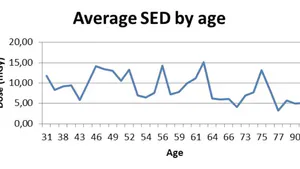
In addition, we determined the behavior of the average dose received by patients, now as a function of their age. The corresponding results are shown in Fig. 7 (SED) and 8 (MGD).
{"image_source":{"path":"images/d11da63c3cb0180062314562932e6411a54abe011c2368bc07bd329ecb33315e.jpg"},"content":"","chart_caption":[{"type":"text","content":"Average SED by age"},{"type":"text","content":"(a)"}],"chart_footnote":[]} {"image_source":{"path":"images/4644fd3a68c72993b78162bb95784e22f7d6733f00a47dd3302f18661a9d1952.jpg"},"content":"","chart_caption":[{"type":"text","content":"(b)"}],"chart_footnote":[]}
{"image_source":{"path":"images/e37547120927482e73e06e546de6e0da787795b977fde3a30d636875011c292a.jpg"},"content":"","chart_caption":[{"type":"text","content":"Average SED by age"},{"type":"text","content":"(c)"},{"type":"text","content":"Fig. 7: Graphical behavior of SED as a Function of the Patients age for the Respective dataset: (a) for UNIT 1; (b) for UNIT 2 and (c) for UNIT 3"}],"chart_footnote":[]} {"image_source":{"path":"images/06d10ff0ce94c672e5d9e4cc38e83306a1bee920df80e3ae3d55f2fcff5c10d9.jpg"},"content":"","chart_caption":[{"type":"text","content":"Average MGD by age"},{"type":"text","content":"(a)"}],"chart_footnote":[]}
{"image_source":{"path":"images/75a15e682f8f48d1f66e57df55b89e18adf318180c9ff205f85cb21c303357a6.jpg"},"content":"","chart_caption":[{"type":"text","content":"Average MGD by age"},{"type":"text","content":"(b)"}],"chart_footnote":[]} {"image_source":{"path":"images/cdfea589363d68bf69ea69c72782e9965619e828af931135e33833b2ac98e231.jpg"},"content":"","chart_caption":[{"type":"text","content":"(c)"},{"type":"text","content":"Fig. 8: Graphical behavior of MGD as a Function of the Patients age for the Respective Dataset: (a) for UNIT 1; (b) for UNIT 2 and (c) for UNIT 3"}],"chart_footnote":[]}
3.2 Determining the Mammography Systems Operating Parameters
Among the data collected in the study, the operating parameters recorded by the equipment (kV and mAs) as well as the systems behavior in terms of target-filter combinations used during the exposures were also considered. The graphs obtained from this evaluation are illustrated in Fig. 9 and 10.
{"image_source":{"path":"images/785e20fbbebdda0174372cc81cc02e615fce115b082d88d21d7d0eea2c4ee380.jpg"},"content":"","chart_caption":[{"type":"text","content":"Average kVp by thickness range (Mo/Mo)"},{"type":"text","content":"(a)"}],"chart_footnote":[]} {"image_source":{"path":"images/445ffb5e971cfeb88a96573ce00711f1521f47c0fb63086071ca5c42cb0213f0.jpg"},"content":"","chart_caption":[{"type":"text","content":"Average mAs (Exp) by thickness range (Mo/Mo)"}],"chart_footnote":[]}
{"image_source":{"path":"images/82212e59a973cc8d06347db24e1ec2713dfb1f6f382ab095998da0a32aafc5ae.jpg"},"content":"","chart_caption":[{"type":"text","content":"Average kVp by thickness range (Mo/Rh)"},{"type":"text","content":"(b)"}],"chart_footnote":[]} {"image_source":{"path":"images/eadf2950b731feaf9462521ec7dc33d986860050d9268354d72c34186abb3999.jpg"},"content":"","chart_caption":[{"type":"text","content":"Average mAs (Exp) by thickness range (Mo/Rh)"}],"chart_footnote":[]}
{"image_source":{"path":"images/1d27a4fb37e3aff290918a64d6bd189b01ba019b20499887bce0984defe062af.jpg"},"content":"","chart_caption":[{"type":"text","content":"Average kVp by thickness range (Rh/Rh)"},{"type":"text","content":"(c)"}],"chart_footnote":[]} {"image_source":{"path":"images/f6e2228f7ff6ee1cf2ed3581cc3a84a82505242236be8a3d4d96848a033894bd.jpg"},"content":"","chart_caption":[{"type":"text","content":"Average mAs (Exp) by thickness range (Rh/Rh)"}],"chart_footnote":[]}
{"image_source":{"path":"images/97732d256bcc81c8546022df9c8306e88aa85dc859203a09d24f227192916b74.jpg"},"content":"","chart_caption":[{"type":"text","content":"Average kVp by thickness range(Mo/Mo)"},{"type":"text","content":"(d)"}],"chart_footnote":[]} {"image_source":{"path":"images/e20933d090bf9a44be9a4fb510ab414ba8d5ce44056424baaa990e08915bc9c3.jpg"},"content":"","chart_caption":[{"type":"text","content":"Average mAs (Exp) by thickness range(Mo/Mo)"}],"chart_footnote":[]}
{"image_source":{"path":"images/dba8c6ae47429d447bd168a0d90f2d2cc8c62609e58148eb141d37d4a82bcd78.jpg"},"content":"","chart_caption":[{"type":"text","content":"Average kVp by thickness range(Mo/Rh)"},{"type":"text","content":"(e)"}],"chart_footnote":[]} {"image_source":{"path":"images/41b475d6da17028395c3f20c59598233bbb186eb8b561e77afb8783b48ac1ee3.jpg"},"content":"","chart_caption":[{"type":"text","content":"Average mAs (Exp) by thickness range (Mo/Rh)"}],"chart_footnote":[]}
{"image_source":{"path":"images/ad81dd6556af51ab6e4c32a1f6ad1fd15c580dcbca31d6e0982f0296073044df.jpg"},"content":"","chart_caption":[{"type":"text","content":"Average kVp by thickness range(Rh/Rh)"},{"type":"text","content":"(f)"}],"chart_footnote":[]} {"image_source":{"path":"images/66af0c1db882cf04cae78d37015cb57a9dfa1adb6ddfd031ae2c613d48b4bda3.jpg"},"content":"","chart_caption":[{"type":"text","content":"Average mAs (Exp) by thickness range (Rh/Rh)"}],"chart_footnote":[]}
{"image_source":{"path":"images/c0184761758a77fbbfc8f7c3393ebd6323e8c03976336fa05b48ec3a8025ec5f.jpg"},"content":"","chart_caption":[{"type":"text","content":"Average kVp by thickness range (Mo/Mo)"},{"type":"text","content":"(g)"}],"chart_footnote":[]} {"image_source":{"path":"images/eafa2468473d45b8cab884298a6f6f1618c78690bfff1c375dbd19ab4c34234f.jpg"},"content":"","chart_caption":[{"type":"text","content":"Average mAs (Exp) by thickness range (Mo/Mo)"}],"chart_footnote":[]}
{"image_source":{"path":"images/47c42b3142bfc18a17c11c0a9384438114e7303a63f16ddabd29fbb546778b6f.jpg"},"content":"","chart_caption":[{"type":"text","content":"Average kVp by thickness range (Mo/Rh)"},{"type":"text","content":"(h)"}],"chart_footnote":[]} {"image_source":{"path":"images/4e74414fc8d9fd6dc7366cc83e713308eb53ce0939ab10a270d6457d85b13c91.jpg"},"content":"","chart_caption":[{"type":"text","content":"Average mAs (Exp) by thickness range (Mo/Rh)"}],"chart_footnote":[]}
{"image_source":{"path":"images/79d1eed39830b60a3285924a07c893b87cf776542769dee6aadc095597d050f7.jpg"},"content":"","chart_caption":[{"type":"text","content":"Average kVp by thickness range (Rh/Rh)"},{"type":"text","content":"(i)"}],"chart_footnote":[]} {"image_source":{"path":"images/0e03216ad34a7948346166a833955e858e4f47d4a8b7434a6a26dbbfc4eaafff.jpg"},"content":"","chart_caption":[{"type":"text","content":"Average mAs (Exp) by thickness range (Rh/Rh)"},{"type":"text","content":"Fig. 9: Average kVp and mAs values by breast thickness ranges during exams for the respective target/filter combinations of the tube: (1) Mo/Mo; (2) Mo/Rh; (3) Rh/Rh. They are illustrated, respectively, as follows: (a), (b) and (c) for UNIT 1; (d), (e) and (f) for UNIT 2; and (g), (h) and (i) for UNIT 3"}],"chart_footnote":[]}
{"image_source":{"path":"images/3882b30f39d0f164b906f2629302ca8a5aee9bc9f9c7c203b7db8cfd6f174f88.jpg"},"content":"","chart_caption":[{"type":"text","content":"Target/filter combination frequency"},{"type":"text","content":"(a)"}],"chart_footnote":[]} {"image_source":{"path":"images/6c2f8dec7a93e27e330ea2eb6f31838668fd0473fe66c465dfa2b081e39e3da0.jpg"},"content":"","chart_caption":[{"type":"text","content":"Target/filter combination frequency"},{"type":"text","content":"(b)"}],"chart_footnote":[]}
{"image_source":{"path":"images/a4dc70401ca14886a787ed16984e73bf6da7e88b7ee5f2ec959d14f6da30982f.jpg"},"content":"","chart_caption":[{"type":"text","content":"Target/filter combination frequency"},{"type":"text","content":"(c)"},{"type":"text","content":"Fig. 10: Percentage of Cases for the Target/filter Combinations used: (a) UNIT 1; (b) UNIT 2; (c) UNIT 3"}],"chart_footnote":[]}
3.3 Determining the Breast Areas and Radiographic Density from the Mammography Images
Additionally to the data shown in the previous sections, we have determined both the sizes of the breast areas relative to those images and the radiographic density of each one by applying the most current version of the LIBRA software (Breast Imaging Group, UPenn) [11] on all image datasets obtained from the 3 mammography Units. Consequently, it was possible to determine the profile of these 3 datasets in terms of radiographic density variation (in BIRADS categories, for example) and the size of breast areas in patients from those centers. This section categories, for example) and the size of breast areas in patients from those centers. This section shows graphical representations illustrating these profiles. The radiographic density profiles by breast projection (CC and MLO) are illustrated in
Fig. 11 (a, b and c, respectively for Units 1, 2 and 3). And Fig. 12 illustrates the profile corresponding to the percentage of patients by the size ranges of breast areas – considering also the two projections (CC and MLO).
{"image_source":{"path":"images/697f450462d820f0bfa1d5f810056b97c7d242a7e1d786835faefea1f71deb31.jpg"},"content":"","chart_caption":[],"chart_footnote":[]} {"image_source":{"path":"images/bdffa8735e26b82ec466cb0fe3cc06bdcbb66cdd5d9b888e0f0ef02ee5701b2a.jpg"},"content":"","chart_caption":[{"type":"text","content":"(a)"},{"type":"text","content":"(b)"}],"chart_footnote":[]}
{"image_source":{"path":"images/ae012aaba1ec247d0ca6509581b2adcee3c0530a8b8a710470ea61582e856f41.jpg"},"content":"","chart_caption":[{"type":"text","content":"Radiographic density frequency (by projection)"},{"type":"text","content":"(c)"},{"type":"text","content":"Fig. 11: Profile of Percentage of Images in the Set in each of the 4 BIRADS Radiographic Density Intervals for both Images Projections (CC and MLO): (a) UNIT 1; (b) UNIT 2; (c) UNIT 3"}],"chart_footnote":[]} {"image_source":{"path":"images/946ef374b8ee761b3ee8962ff33cb95a7af8696c83ee98b0638b305dcaf08b46.jpg"},"content":"","chart_caption":[{"type":"text","content":"% of patients by size ranges of breast areas"},{"type":"text","content":"(a)"}],"chart_footnote":[]}
{"image_source":{"path":"images/ad672fda20e5fd1f377ed6caf07c8e12bda304f4e75dc7fd37d59c59a1bcb2ec.jpg"},"content":"","chart_caption":[{"type":"text","content":"% of patients by size ranges of breast areas"},{"type":"text","content":"(b)"}],"chart_footnote":[]} {"image_source":{"path":"images/77567102e797dec5d05944565b545632b10c09a9d3a906d104d2e6c819128f7c.jpg"},"content":"","chart_caption":[{"type":"text","content":"% of patients by size ranges of breast areas"},{"type":"text","content":"(c)"},{"type":"text","content":"Fig. 12: Profile of Percentage of Patients in each dataset in 6 Ranges of Average breast area size, Considering the CC and MLO Projections: (a) UNIT 1; (b) UNIT 2; (c) UNIT 3"}],"chart_footnote":[]}
IV. DISCUSSION
The dataset acquired in this study was quite extensive, and the data acquisition process for subsequent analysis was significantly facilitated by the storage capabilities provided by the ReadDICOM program . Firstly we primarily focus on the dose profile generated by the systems, along with other statistically relevant profiles of interest to radiology services administration. Regarding the time required for processing and obtaining the base spreadsheet, it was found that the survey for the most extensive image set (1,367 images) took less than 1 minute.
The following subsections will present many comparisons between the 3 systems involved in this investigation, based on the data extracted from the DICOM files recorded and graphically presented in the previous section.
4.1 Comparison of Population Profiles
The primary findings from the comparison of sets of patients undergoing examinations in the three investigated systems are as follows:
a) The average age of patients in the respective groups is approximately 50-60 years, with mean ages of 59, 57 and 52 years for individuals undergoing exams in radiological services of Units 1, 2 and 3, respectively;
b) The average breast thickness, as subjected to examinations, notably exceeds the conventional recommendations typically employed in quality control and phantoms tests (which typically employ an average thickness of 45mm for a breast with 50/50% fibro glandular/adipose tissue): nearly 49mm for Unit 1 group, 56mm for the Unit 2 group, and remarkably, 62.5mm for patients submitted to exams in Unit 3.
These data hold significant implications. They suggest a potential need for healthcare professionals responsible for these services to reevaluate examination procedures and closely observe radiation dose levels produced by the equipment, as this factor is highly dependent on breast thickness during exposure. Moreover, these insights offer valuable directions for the development of techniques and phantoms aimed at quality assessment of the imaging systems. It is also noteworthy that these findings characterize the population profile served by these public radiology services, encompassing both routine and diagnostic examinations.
4.2 Dosimetry Profiles
The ability to swiftly and easily survey dosimetry profiles for each set of equipment through this application represents a significant advantage in terms of a quality evaluation tool for system performance. In a general overview based on the various graphs for each set, the behavior of all three systems aligned with expectations.
Since the most critical aspects of mammography quality control are currently centered on Mean Glandular Dose (MGD), we will not extensively explore the results of Skin Entrance Dose (SED). It is worth noting that, on average, SED records lower values for the mammography Units 1 and 3 (often falling below 9.0 mGy, except for very thick breasts exceeding 80mm, especially in the latter). Conversely, for the Unit 2 equipment, SED reaches 10 mGy or higher for breast thicknesses above 60mm. Even so, data from all Units are satisfactorily reporting average SED around 8.0-9.0%, as shown in Table 1. Still considering the results summarized in that Table, only for Unit 1 data show that worryingly more than 50% of the patients in the group under study received SED above the average value. For the other two mammography services, these numbers were between 38 and 42%. Even so, the proportion of patients who received a SED exceeding the average value plus the calculated standard deviation, relative to the total number of patients, remained below 13% for Units 2 and 3. In contrast, for Unit 1, it was slightly higher, approximately around 18%. These numbers may be attributed to cases where multiple breast exposures were required for clinical reasons.
Regarding the MGD profiles for the three units, two comparisons are of interest: one relative to the recorded values compared to the recommendations outlined in norms and guidelines; and the other comparing the values recorded among the three units (since all correspond to similar models from the same manufacturer). Therefore, from an initial analysis of the graphs presented in Figure 5:
a) Mammography Unit 1 exhibited MGD levels within the acceptable range according to international standards. However, it is worth noting that the lower thickness ranges exhibit average MGD values approximately 50% higher than both the acceptable and desirable values, with values reaching the upper limits for the next range (41-50 mm) and falling below the "limits" for the larger thickness ranges. It is important to note that, for this equipment, the majority of patients had breast thicknesses ranging from 43 to 60 mm (Figure 1), encompassing 435 images within this interval, and their average MGD values align with the standards. Furthermore, instances where slightly elevated MGD is recorded in the lower thickness ranges are associated with low absolute values (around 1.5 mGy).
b) A similar pattern is observed in the analysis of the graph presented for the mammography Unit 2. Once again, the average MGD values recorded for the lower thickness ranges (21-30 mm and 31-40 mm) were in close proximity to their respective limits. When compared to the "desirable" values, which are adopted by Brazilian standards and are more restrictive, it becomes evident that they are slightly higher (approximately 20% higher in the lower thickness range and up to 50% higher between 31-40 mm). For the other thickness ranges, the MGD levels are comfortably below both the acceptable and desirable limits as outlined in the standards.
c) The mammography Unit 3 demonstrates a more consistent alignment with international standards in terms of average MGD values. The only exception is the 31-40 mm thickness range, where the recorded MGD reaches 2.0 mGy (compared to an "acceptable" value of 1.5 mGy and a "desirable" value of 1.0 mGy). However, this particular observation, while warranting some attention, does not appear to be significantly concerning. This is due to the fact that the majority of patients in the dataset had breast thicknesses ranging from 50 to 74 mm, encompassing 930 images in the evaluated group, with average MGD values well below both the acceptable and desirable limits.
d) It is noteworthy that the primary MGD distribution ranges for each equipment are as follows: for Unit 1, they range from 1.8 to 2.4 mGy; for the mammography Unit 2, they fall between 1.0 and 2.0 mGy; and for Unit 3, they extend from 1.2 to 1.8 mGy. Additionally, there is a notable subset within the Unit 3 distribution that falls between 2.2 and 2.6 mGy, primarily attributable to the group with the thickest breasts among all the analyzed.
e) In comparative terms, the MGD profiles for all three Units exhibit remarkable similarity, particularly between the Units 2 and 3, whose overall MGD profiles closely resemble each other despite differences in the number of cases/patients included. The MGD profile for Unit 1, on the other hand, displays a slight divergence, characterized by an unexpected decrease in dose values for thicker breasts. Unfortunately, further comparisons with this equipment are no longer feasible, as the corresponding radiology service has replaced it with a new different system capable of performing breast tomosynthesis exams.
It is also of interest to note that the average values of SED and MGD tend to decrease with the patients age (according to Fig. 7 and 8). It is worth highlighting that those profiles show that the average MGD for all age groups within each set remains consistently limited in the range of 1.0 to 2.5 mGy for Unit 2 set, with minor variations in the lower limits for the other systems (1.5-2.5 mGy for Unit 1 and 1.2-2.5 mGy for Unit 3). This confirms the primary results of average MGD by patients shown earlier in Table 1.
4.3 X-ray Spectrum Profiles
The graphs presented in Figure 9 illustrate operational parameter profiles of the mammography systems, specifically in relation to the target/filter combinations used during examinations. These profiles are depicted across various breast thickness ranges exposed to the systems. Notably, there are certain similarities among the three systems:
a) For the Mo/Mo target/filter combination, all three systems exhibit nearly constant behavior, maintaining an average energy level of approximately 26 kVp across all breast thickness ranges.
b) Similarly, for the Rh/Rh target/filter combination, all three systems operate within a range of 29 to 30 kVp across different thickness ranges. However, it's worth mentioning that the mammography Units 2 and 3 reach 30 kVp primarily for very thick breast tissue (above 70mm).
c) In contrast, for the Mo/Rh target/filter combination, there is a noticeable difference. The Units 1 and 3 operate with energy levels between 26 and 27 kVp. In contrast, Unit 2 exhibits a higher energy profile, operating between 29 and 30 kVp. This variance may be an adjustment to compensate for the fact that, within this same combination, the Exposure (mAs) value recorded by the Unit 2 system is considerably lower compared to the other two. Unit 2 records exposures between 64 and 72 mAs, while the other two systems show a broader range, varying from 60 to 100 mAs (Unit 1) and 50 to even 200 mAs, especially for breast thickness ranges above 70mm, in the case of Unit 3.
The operational parameter profiles also reveal significant differences in the recorded values across the three sets. Notably, for the Mo/Mo combination, the Unit 3 set maintains a nearly constant exposure level of around 200 mAs. In contrast, the Unit 2 set does not exceed 100 mAs, and the Unit 1 set records even lower values, ranging from 40 to 80 mAs. These differences can be attributed to the typical breast thicknesses and densities registered in each set's patient population, with the group corresponding to Unit 3 characterized by notably thicker breast tissue.
However, it is important to note that a more comprehensive comparison can be made by considering the most frequently used condition, which is the Rh/Rh target/filter combination. Remarkably, between 70% and 80% of all images in the analyzed datasets were produced using the Rh/Rh combination. This observation aligns with expectations, especially in the case of the Unit 3 dataset, where higher average breast thicknesses are registered.
In the comparison of profiles across the three groups, one notable difference is the recorded mAs values in the Unit 1 group. Interestingly, a decline in mAs values is observed as breast thickness increases, ranging from 120 mAs for thicknesses in the 31-40mm range to approximately 80 mAs for thicknesses above 70mm. In contrast, both the mammography units 2 and 3 exhibit a different pattern, which is relatively consistent between them. These systems show increasing mAs values as breast thickness ranges increase, ranging from 60 to 140 mAs for the former and from 50 to 170 mAs for the latter. This behavior aligns with expectations for these cases, where higher breast thickness typically requires higher exposure settings to maintain image quality.
This distinction in mAs behavior among the groups may reflect variations in patient populations, breast tissue characteristics, or specific clinical practices at each radiology service, featuring the importance of considering these factors in dose optimization and quality control efforts.
4.4 Radiographic Density Profiles
The analyses performed so far have been based on the use of the software previously developed applied to the image datasets under consideration. We complemented this analysis by leveraging the LIBRA software (Breast Imaging Group, UPenn) . This freely accessible software provides, in addition to the original and segmented images and a histogram of the analysis, three essential pieces of information: the size (in cm ) of the total area of the cropped breast, the size (also in cm ) of the segmented area, and the ratio (expressed as a percentage) between them, which the program defines as the radiographic density of the breast. These data, along with other attributes related to each image (such as whether it is a CC or MLO projection, left or right, etc), are recorded within a spreadsheet. The information derived from LIBRA led to additional graphical representations documented in Fig. 11 and 12, focusing on the relationships among the Average Radiographic Density per patient, the percentage of cases within the four classic density intervals defined by BIRADS, as well as the average and maximum breast area sizes, considering MLO and CC projections.
From these graphs, it is interesting to highlight an observation: in all of them, according to LIBRA results, the overwhelming majority of patients undergoing examinations are in BIRADS category A, i.e., breasts with radiographic densities lower than 25% (almost 90% of cases for Units 1 and 2 sets, and almost 80% for Unit 3 set). The groups corresponding to category B (densities between 25 and 50%) practically complete the sets, representing about 10% of cases. Tests with an older version of that program did not change this result, which, however, is somewhat surprising since it does not exactly reflect what is usually observed in radiology routine (where there is a greater distribution of cases between densities up to 75%, at least) and therefore deserves further investigation.
Regarding breast area profiles, it is interesting to note that these data complement well the results related to the average breast thicknesses of the patients examined in each of those services. They show that the majority of patients have breast areas ranging from 100 to 200 cm . In more detail: (a) from the Unit 1 set, just over 30% correspond to areas of 100 to 150 cm , another 30% have an area smaller than 100 cm , and 23% are between 150 and 200 cm ; (b) from the Unit 2 set, 40% of breasts are in the range of 100 to 150 cm (21% are smaller than 100 cm , and 22% are between 150 and 200 cm ); and (c) from the Unit 3 set, about 33% are between 100 and 150 cm , and another 28% are between 150 and 200 cm .
V. CONCLUSION
The DICOM header information included in the images is a valuable asset for the study outlined in this article. The extensive data stored within the image files played an essential role in establishing profiles with meaningful correlations and outcomes regarding patient demographics, radiation doses they were exposed to, and parameters of the hospital's mammography system. The use of the previously developed ReadDICOM tool significantly streamlined this process.
It is important to note that, despite the extensive number of exposures included in this study, certain instances with smaller sample sizes (such as extreme cases of age or breast thickness or less commonly used target/filter combinations) exhibited biased results. Consequently, for future extensions of the study, increasing the number of exposures would be useful to enable a more comprehensive and representative analysis of the patient population in a particular radiological service. Additionally, for supplementary investigations, incorporating exposures from different models of digital mammography equipment could yield valuable insights into radiation doses and operational parameters.
In our particular study, three important aspects could be highlighted based on the analysis of population profiles and dose records in the investigated radiological services. The average breast thickness ranged from approximately 50mm to 62mm, depending on the radiology service considered, indicating values above what is typically used as a standard for conventional quality assurance programs (e.g., in phantoms used for tests). The average age of the patients ranged from 52 to 60 years, indicating a prevalence of non-elderly women in the evaluated group. Despite this, the analysis of radiographic density of the images showed a significant presence of BIRADS A cases in the same group (even for the mammographic Unit corresponding to the population with the lowest average age).
Finally, all the equipment produced average glandular dose profiles within the limits recommended by international standards and norms – although in some cases there were occasional "deviations", almost always due to thicker breasts. This is an important conclusion as it demonstrates that the present work, through the scan obtained by the ReadDICOM application, rapidly and practically detected the dosimetry profiles of each investigated mammography equipment, enabling its use to optimize the management process of their respective radiological services.
In conclusion, the significance of analyses like the one conducted in this investigation cannot be overstated. As previously emphasized, mammography examinations play a primary role in the early detection of breast cancer, and should be conducted routinely throughout a woman's adult life. Hence, comprehending the patient population profiles and the radiation doses they are exposed to during these examinations is valuable – especially for the management of the mammography service. In fact, having access to information such as those presented in this study makes it easier to implement progressively substantial safety measures to the process.
ACKNOWLEDGEMENTS
The authors are thankful to FAPESP for the financial support, and also to the Management of Education & Research of University Hospital of Federal University of São Carlos (SP, Brazil) - Brazilian Company of Hospital Services (EBSERH).
Conflict of Interest
The authors declare no conflict of interest.
Ethical Approval
Not applicable
Data Availability
The datasets used in this study are openly available at [repository link] and the source code is available on GitHub at [GitHub link].
Funding
This work did not receive any external funding.
References
Cite this article
Related Research


Special Issue
Launch a focused special issue to highlight research, emerging trends, and expert insights in your academic field.
