I. INTRODUCTION
Spectral dichotomy methods were introduced by S. K. Godunov in [6] for the study of stability in the sense of Lyapunov. They consist in determining whether or not there are eigenvalues of a given matrix or a matrix pencil inside or outside a closed contour. If there are no eigenvalues in a neighborhood of the contour, these methods compute iteratevely the projector onto the invariant subspace associated to the eigenvalues of the matrix or the matrix pencil inside the contour. This computation is accompanied by the spectral norm of a Hermitian positive definite matrix H called the dichotomy condition number. Initially developed on the imaginary axis by S. K. Godunov [6], these methods have been extended to the circle by Bulkgakov and Godunov in [2]. More efficient methods for computing the spectral projector and the dichotomy matrix in the circular case were proposed by Malyshev in [11, 12], Sadkane and Dosso in [4], Sadkane and Touhami in [17]. The methods of spectral dichotomy of a matrix or a matrix pencil with respect to the ellipse or parabola are respectively transformations of the methods with respect to the circle or imaginary axis. The methods with respect to the ellipse have been proposed by Godunov and Sadkane in [8, 9], Malyshev and sadkane in [14] and Sadkane and Touhami in [17] and those with respect to the parabola by Malyshev and sadkane in [14] and Sadkane and Touhami in [17]. Traoré et al. in [19, 20, 18] applied the dichotomy methods of a matrix with respect to the circle, the ellipse and the parabola all not centered at the origin.
Let be a regular matrix pencil with and with non singular. The aim of this paper is to propose some methods of spectral dichotomy of the matrix pencil with respect to the circle of center with affix and radius , the ellipse of equation
\[\left(\frac{x - x_0}{a}\right)^2 + \left(\frac{y - y_0}{b}\right)^2 = 1, \quad a \geq b > 0\]
and of center different from 0 and the parabola of equation
\[2p(d-x)=(y-p\tilde{b})^2\]
with p > 0.
(1.2)
Our work is organized as follows. In the section 2, we recall the spectral dichotomy methods of a matrix pencil with respect to the circle and the ellipse [16], all centered at the origin and with respect to the imaginary axis [16]. Algorithms developed in this section are useful for the sequel. In section 3, we propose new algorithms to compute the spectral projector and dichotomy matrix of a matrix pencil with respect to a circle, an ellipse or a parabola off centered at the origin. In this section, we use special matrix pencils to bring us back to the algorithms seen in the section 2. In section 4, we illustrate our results using graphs and tables to visualise and demonstrate the accuracy of our algorithms.
Throughout this work, we will use the following notation: the symbol denotes the 2-norm for vectors and matrices. The identity matrix (respectively the null matrix) of order will be denoted by (respectively ) or just (respectively 0) if the order is clear from the context.
II. SOME METHODS OF SPECTRAL DICHOTOMY OF A MATRIX PENCIL
Let be a matrix pencil with , , .
2.1 Method of spectral dichotomy of a matrix pencil with respect to a circle centered at the origin
Suppose that the matrix pencil has no eigenvalue in a circle , . Then
\[\mathbb{P} = \frac{1}{2\pi} \int_0^{2\pi} \left(B - e^{-i\theta} \frac{A}{r}\right)^{-1} B d\theta\]
is a spectral projector onto the subspace corresponding to the eigenvalues of inside the circle .
The numerical computation of P is accompanied by the dichotomy condition number given by the spectral norm of the Hermitian positive definite matrix
\[\mathbb{H} = \frac{1}{2\pi} \int_0^{2\pi} \left(B - e^{-i\theta} \frac{A}{r}\right)^{-*} \mathbb{H}^0 \left(B - e^{-i\theta} \frac{A}{r}\right)^{-1} d\theta\]
where is a given arbitrary matrix.
Consider the cyclic and finite linear system [8]
\[\left\{ \begin{array}{l l} B Z _ {0} ^ {(2 ^ {j})} - \frac {A}{r} Z _ {1} ^ {(2 ^ {j})} & = I _ {n}, \\ B Z _ {k} ^ {(2 ^ {j})} - \frac {A}{r} Z _ {k + 1} ^ {(2 ^ {j})} & = 0, \qquad 1 \leq k \leq 2 ^ {j} - 1. \end{array} \right.\tag{2.3}\]
From its solutions , the following theorem allows to obtain the values of and (see [8, 16]).
Theorem 2.1 We have
\[\mathbb {P} = \lim _ {j \to + \infty} \mathbb {P} _ {j} \qquad w i t h \quad \mathbb {P} _ {j} = Z _ {2 j} ^ {(2 ^ {j})} B \equiv Z _ {0} ^ {(2 ^ {j})} B\tag{2.4}\]
and
\[\mathbb{H} = \lim_{j \to +\infty} \mathbb{H}_{j} \quad \text{with} \quad \mathbb{H}_{j} = \sum_{k=1} (Z_{k}^{(2^{j})})^* \mathbb{H}^{0}(Z_{k}^{(2^{j})}),\]
\[\mathbb{H}_{j} = V_{j}^* \mathbb{H}_{j-1} V_{j} + W_{j}^* \mathbb{H}_{j-1} W_{j}\]
where and .
As for the computation of and , they are explained in the following theorem (see [16])
Theorem 2.2 Let
\[Z _ {1} ^ {(2)} = \Delta_ {0}, Z _ {2} ^ {(2)} = \nabla_ {0}\]
and for
\[Z _ {k} ^ {(2 ^ {j})} = Z _ {k} ^ {(2 ^ {j - 1})} \Delta_ {j - 1}, k = 1, 2, \dots 2 ^ {j - 1}.\]
\[Z _ {k + 2 ^ {j - 1}} ^ {(2 ^ {j})} = Z _ {k + 2 ^ {j - 1}} ^ {(2 ^ {j - 1})} \nabla_ {j - 1}, k = 1, 2, \dots 2 ^ {j - 1}.\]
and for
\[A _ {j - 1} + B _ {j - 1} = I _ {n}\tag{2.7}\]
\[\Delta_{j-1} + \nabla_{j-1} = I_n\tag{2.8}\]
\[(2 A _ {j - 1} - I _ {n}) \Delta_ {j - 1} = A _ {j - 1}\tag{2.9}\]
with
\[A_{j-1} = -\frac{A}{r} Z_1^{(2^{j-1})}, I_n = -Z_1^{(2^{j-1})}\]
\[H_{j} = \Delta_{j-1}^{*} H_{j-1} \Delta_{j-1} + (I_{n} - \Delta_{j-1})^{*} H_{j-1} (I_{n} - \Delta_{j-1}).\]
Following Algorithm 2.1 given in [17] summarizes the computations of the projector P and the dichotomy criterion .
Algorithm 2.1
Input: such the matrix pencil is regular having no eigenvalues on the circle , .
used for scaling.
Output: the projector onto the subspace of associated with the eigenvalues inside the circle , .
the integral whose norm indicates the numerical quality of the projector .
1. Initialisation and first iteration
\[H _ {0} = H ^ {0} \qquad and \quad \tilde{A} = \frac{A}{r}\]
- Determine the solutions of equations
\[X (B - \tilde {A}) = \tilde {A}, Y (B - \tilde {A}) = I\]
- Determine the solutions of equations
\[(\tilde {A} + B) \Delta_ {0} = X, (\tilde {A} + B) \nabla_ {0} = Y\]
\[\begin{array}{r} H _ {1} = \Delta_ {0} ^ {*} H _ {0} \Delta + \nabla_ {0} ^ {*} H _ {0} \nabla_ {0} \\Z _ {1} ^ {2} = \Delta_ {0}, \quad Z _ {2} ^ {(2)} = \nabla_ {0} \end{array}\] 2. Iterations for
\[A _ {j - 1} = - \tilde {A} Z _ {1} ^ {2 ^ {j - 1}}\]
\[(2 A _ {j - 1} - I _ {n}) \Delta_ {j - 1} = A _ {j - 1}\]
\[H _ {j} = \Delta_ {j - 1} ^ {*} H _ {j - 1} \Delta_ {j - 1} + (I - \Delta_ {j - 1}) ^ {*} H _ {j - 1} (I _ {n} - \Delta_ {j - 1})\]
\[Z _ {1} ^ {(2 ^ {j})} = Z _ {1} ^ {(2 ^ {j - 1})} \Delta_ {j - 1}, Z _ {2 ^ {j}} ^ {(2 ^ {j})} = Z _ {2 ^ {j - 1}} ^ {(2 ^ {j - 1})} (I _ {n} - \Delta_ {j - 1})\]
end for
\[\mathbb{P} _ {0} = Z _ {2 ^ {j}} ^ {(2 ^ {j})} \qquad and \qquad \mathbb{H} = H _ {j}\]
2.2 Method of spectral dichotomy of a matrix pencil with respect to an ellipse centered at the origin
Suppose that the matrix pencil has no eigenvalues on the ellipse of equation
\[\left(\frac{x}{a}\right)^{2} + \left(\frac{y}{b}\right)^{2} = 1 \quad \text{with} \quad a \geq b > 0.\]
Consider the matrix pencil of the form where
\[\mathcal {B} = \left( \begin{array}{c c} \frac {a + b}{2} B & - A \\0 & \frac {a + b}{2} B \end{array} \right) \qquad \text {and} \quad \mathcal {A} = \left( \begin{array}{c c} - \frac {a - b}{2} B & 0 \\A & - \frac {a - b}{2} B \end{array} \right)\tag{2.11}\]
This following proposition shows the dichotomy parameters
\[\alpha = \sup _ {z \in \Xi_ {z _ {0}}} \| (z I _ {n} - A) ^ {- 1} \| \quad \text { and } \quad \widetilde {\alpha} = \sup _ {| \widetilde {\lambda} | = 1} \| (\widetilde {\lambda} \widetilde {\mathcal {B}} - \widetilde {\mathcal {A}}) ^ {- 1} \|\tag{2.12}\]
are equal.
Proposition 2.1 Let and defined in (3.5). then
\[\alpha = \widetilde{\alpha}.\]
Moreover, if we denote by
\[\mathcal{P}_{\infty} = \left( \begin{array}{c c} \widetilde{\mathcal{P}}_{1 1} & \widetilde{\mathcal{P}}_{1 2} \\\widetilde{\mathcal{P}}_{2 1} & \widetilde{\mathcal{P}}_{2 2} \end{array} \right), \quad \text{with} \quad \widetilde{\mathcal{P}}_{i j} \in \mathbb{C}^{n \times n}, \quad i, j \in 1, 2.\tag{2.14}\]
the projector onto the invariant subspace of the matrix pencil associated with the eigenvalues inside and the projector onto the invariant subspace of the matrix pencil associated with the eigenvalues inside .
The following proposition characterizes the relation between and .
Proposition 2.2 We have
\[\mathbb{P}_{\infty} = \widetilde{\mathcal{P}}_{11} + \widetilde{\mathcal{P}}_{22}.\]
Following Algorithm 2.2 given in [17] summarizes the computations of the projector and the dichotomy criterion .
Algorithm 2.2.
being the projector on the right invariant space of corresponding to the eigenvalues outside the ellipse and the dichotomy criterion.
1. Set
\[\mathcal{B} = \left( \begin{array}{c c} \frac{a + b}{2} B & - A \\0 & \frac{a + b}{2} B \end{array} \right) \quad and \quad \mathcal{A} = \left( \begin{array}{c c} - \frac{a - b}{2} B & 0 \\A & - \frac{a - b}{2} B \end{array} \right)\tag{2.16}\]
2. Apply algorithm 2.1 to
3. We obtain and H.
2.3 Method of spectral dichotomy of a matrix pencil with respect to an imaginary axis
Suppose that the matrix pencil has no eigenvalues on the imaginary axis. Consider the matrix pencil where and . This following proposition shows the relation between the dichotomy parameters
\[\widetilde {\alpha} = \sup _ {| \lambda | = 1} \| \lambda \mathcal {B} - \mathcal {A}) ^ {- 1} \| \quad \text { and } \quad \alpha = \sup _ {\Re z = 0} \| (z B - A) ^ {- 1} \|\tag{2.17}\]
Proposition 2.3 [17] Assume that and let and be the two parameters defined in (2.17)
\[\frac {1}{2} \alpha \leq \widetilde {\alpha} \leq C (\alpha + 1)\tag{2.18}\]
with
Following Algorithm 2.3 given in [16, 17] summarizes the computations of the projector and the dichotomy criterion .
Algorithm 2.3:
being the projector on the invariant subspace of corresponding to the eigenvalues of negative real parts and the dichotomy criterion.
-
Determine the matrices and .
-
Apply Algorithm 2.1 to .
3.
III. SPECTRAL DICHOTOMY METHODS OF A MATRIX PENCIL WITH RESPECT TO AN OFF-CENTER
Let be a matrix pencil with , such that is not singular.
3.1 Spectral dichotomy method of a matrix pencil with respect to a circle not c entered at the origin
If the matrix pencil has no eigenvalues on the circle ; , then the spectral projector on the invariant subspace corresponding to the eigenvalues on the disc is the matrix defined by:
\[\begin{array}{l l l} \mathbb{P} _ {0} & = & \frac{1}{2 i \pi} \int_ {\mathcal{C} (\Omega , r)} (z B - A) ^ {- 1} B d z \\& = & \frac{1}{2 i \pi} \int_ {| z - b | = r} (z B - A) ^ {- 1} B d z \\& = & \frac{1}{2 i \pi} \int_ {0} ^ {2 \pi} \left((b + r e ^ {i \theta}) B - A\right) ^ {- 1} B i r e ^ {i \theta} d \theta \\& = & \frac{1}{2 \pi} \int_ {0} ^ {2 \pi} \left(B + \frac{b B - A}{r} e ^ {- i \theta}\right) ^ {- 1} B d \theta \\& = & \frac{1}{2 \pi} \int_ {0} ^ {2 \pi} \left(B - \frac{\mathcal{A}}{r} e ^ {- i \theta}\right) ^ {- 1} B d \theta \end{array}\]
where .
The computation of the spectral projector is accompanied by that of a Hermitian matrix defined by:
\[\mathbb{H} = H(r) = \frac{1}{2\pi} \int_0^{2\pi} \left(B - \frac{e^{-i\theta}\mathcal{A}}{r}\right)^{-*} H^{(0)} \left(B - \frac{e^{-i\theta}\mathcal{A}}{r}\right)^{-1} d\theta ,\]
where is a positive definite Hermitian matrix used for setting purposes the scale. We have the following algorithm that compute the projector onto the invariant subspace of corresponding to the eigenvalues inside the circle and the Hermitian and definite positive matrix associated.
Algorithm 3.1.
being the projector on the invariant space of corresponding to the eigenvalues inside the circle and the matrix integral whose norm indicates the quality of the projector .
-
Determine the matrix .
-
Compute the projector and the matrix by applying Algorithm 2.1 to the matrix and to the circle with center and radius .
3.2 Spectral dichotomy method of a matrix pencil with respect to an ellipse not centered at the origin
Consider the ellipse
\[\Xi_ {z _ {0}} = \left\{z = x + i y \in \mathbb {C} \quad | \quad (x - x _ {0}) + i (y - y _ {0}) \in \Xi_ {0} \right\}\tag{3.2}\]
of equation (1.1).
Suppose that the matrix pencil has no eigenvalues on the ellipse . Consider the matrices of order defined in the following way:
\[\widetilde {\mathcal {B}} = \left[ \begin{array}{c c} \frac {a + b}{2} B & - A _ {0} \\0 & \frac {a + b}{2} B \end{array} \right] \qquad \text {and} \quad \widetilde {\mathcal {A}} = \left[ \begin{array}{c c} - \frac {a - b}{2} B & 0 \\A _ {0} & - \frac {a - b}{2} B \end{array} \right]\tag{3.3}\]
where .
The eigenvalues of the matrix pencil and of the matrix pencil are linked by the relation (3.4).
\[\widetilde{z} = \frac{(a + b)\widetilde{\lambda}^{2} + (a - b)}{2\widetilde{\lambda}}\]
Consider the qualities of the spectral dichotomy with respect to the ellipse and the unit circle respectively defined by
\[\alpha = \sup _ {z \in \Xi_ {z _ {0}}} \| (z B - A) ^ {- 1} \quad \text { and } \quad \widetilde {\alpha} = \sup _ {| \widetilde {\lambda} | = 1} \| (\widetilde {\lambda} \widetilde {\mathcal {B}} - \widetilde {\mathcal {A}}) ^ {- 1} \|\tag{3.5}\]
Proposition 3.1 Let and be the quantities defined in (3.5). then
\[\alpha = \widetilde {\alpha}\]
Proof
(3.6) From (3.4), we have
\[\widetilde{z} = \frac{(a + b) \widetilde{\lambda}^{2} + (a - b)}{2 \widetilde{\lambda}}.\]
Which leads to
\[\frac {a + b}{2} B \widetilde {\lambda} ^ {2} - A _ {0} \widetilde {\lambda} + \frac {a - b}{2} B = \widetilde {\lambda} (\widetilde {z} B - A _ {0})\]
We have
\[(\mu^{2} \widetilde{\mathcal{B}} - \widetilde{\mathcal{A}})^{-1} = \left( \begin{array}{cc} (\frac{a + b}{2} \mu^{2} + \frac{a - b}{2}) B & - \mu^{2} A_{0} \\- A_{0} & (\frac{a + b}{2} \mu^{2} + \frac{a - b}{2}) B \end{array} \right)^{-1}\]
\[= \left( \begin{array}{cc} \widetilde{z} \mu B & - \mu^{2} A_{0} \\- A_{0} & \widetilde{z} \mu B \end{array} \right)^{-1}\]
\[= \left( \begin{array}{c c} I _ {n} & 0 \\0 & \mu^ {- 1} I _ {n} \end{array} \right) \left( \begin{array}{c c} \widetilde{z} B & - A _ {0} \\- A _ {0} & \widetilde{z} B \end{array} \right) ^ {- 1} \left( \begin{array}{c c} \mu^ {- 1} I _ {n} & 0 \\0 & I _ {n} \end{array} \right) \\= \left( \begin{array}{c c} I _ {n} & 0 \\0 & \mu^ {- 1} I _ {n} \end{array} \right) \times \\\frac{1}{2} \left[ \begin{array}{c c} (\widetilde{z} B - A _ {0}) ^ {- 1} + (\widetilde{z} B + A _ {0}) ^ {- 1} & (\widetilde{z} B - A _ {0}) ^ {- 1} - (\widetilde{z} B + A _ {0}) ^ {- 1} \\(\widetilde{z} B - A _ {0}) ^ {- 1} - (\widetilde{z} B + A _ {0}) ^ {- 1} & (\widetilde{z} B - A _ {0}) ^ {- 1} + (\widetilde{z} B + A _ {0}) ^ {- 1} \end{array} \right] \\\times \left( \begin{array}{c c} \mu^ {- 1} I _ {n} & 0 \\0 & I _ {n} \end{array} \right) \\= \underbrace{\left( \begin{array}{c c} I _ {n} & 0 \\0 & \mu^ {- 1} I _ {n} \end{array} \right) \left( \begin{array}{c c} \frac{I _ {n}}{\sqrt{2}} & - \frac{I _ {n}}{\sqrt{2}} \\\frac{I _ {n}}{\sqrt{2}} & \frac{I _ {n}}{\sqrt{2}} \end{array} \right)} _ {K _ {1}} \times \left[ \begin{array}{c c} (\widetilde{z} B - A _ {0}) ^ {- 1} & 0 \\0 & (\widetilde{z} B + A _ {0}) ^ {- 1} \end{array} \right] \times \\\underbrace{\left( \begin{array}{c c} \frac{I _ {n}}{\sqrt{2}} & \frac{I _ {n}}{\sqrt{2}} \\- \frac{I _ {n}}{\sqrt{2}} & \frac{I _ {n}}{\sqrt{2}} \end{array} \right)} _ {K _ {2}}\]
\[\sup _ {z \in \Xi_ {0}} \| (\widetilde{z} B - A _ {0}) ^ {- 1} \| = \sup _ {| \widetilde{\lambda} | = 1} \| (\widetilde{\lambda} \widetilde{\mathcal{B}} - \widetilde{\mathcal{A}}) ^ {- 1} \|\]
We notice that the product . Therefore, with a double inequality, we deduce:
We also know that , so we can conclude that
\[\sup _ {z \in \Xi_ {z _ {0}}} \| (z B - A) ^ {- 1} \| = \sup _ {| \widetilde {\lambda} | = 1} \| (\widetilde {\lambda} \widetilde {\mathcal {B}} - \widetilde {\mathcal {A}}) ^ {- 1} \|\]
whence the equality (3.6).
Moreover, if we denote by
\[\mathcal{P}_{\infty} = \left( \begin{array}{c c} \widetilde{\mathcal{P}}_{1 1} & \widetilde{\mathcal{P}}_{1 2} \\\widetilde{\mathcal{P}}_{2 1} & \widetilde{\mathcal{P}}_{2 2} \end{array} \right) \quad \text{with} \quad \mathcal{P}_{i j} \in \mathbb{C}^{n \times n}, i, j = 1, 2.\]
the projector associated with the eigenvalues of the matrix pencil outside the unit circle and the projector associated with the eigenvalues of the matrix pencil inside .
The following proposition characterizes the link between and .
Proposition 3.2 we have
\[\mathbb{P}_{\infty} = \widetilde{\mathcal{P}}_{11} + \widetilde{\mathcal{P}}_{22}\]
\[\begin{array}{r l} & {\left[ \begin{array}{l l} \frac {a - b}{2} B & 0 \\- A _ {0} & \frac {a - b}{2} B \end{array} \right] \left[ \begin{array}{l l} \widetilde {X} & \widetilde {X} _ {1} \\I _ {n} & I _ {n} \end{array} \right]} \\& {+ \left[ \begin{array}{l l} \frac {a + b}{2} B & - A _ {0} \\0 & \frac {a + b}{2} B \end{array} \right] \left[ \begin{array}{l l} \widetilde {X} & \widetilde {X} _ {1} \\I _ {n} & I _ {n} \end{array} \right] \left[ \begin{array}{l l} \widetilde {X} ^ {2} & 0 \\0 & \widetilde {X} _ {1} ^ {2} \end{array} \right]} \\& {= \left[ \begin{array}{c c} \frac {a - b}{2} \widetilde {X} & \frac {a - b}{2} \widetilde {X} _ {1} \\- A _ {0} \widetilde {X} + \frac {a - b}{2} I _ {n} & - A _ {0} \widetilde {X} _ {1} + \frac {a - b}{2} I _ {n} \end{array} \right] + \left[ \begin{array}{c c} (\frac {a + b}{2} \widetilde {X} - A _ {0}) \widetilde {X} ^ {2} & (\frac {a + b}{2} \widetilde {X} _ {1} - A _ {0}) \widetilde {X} _ {1} ^ {2} \\\frac {a + b}{2} \widetilde {X} ^ {2} & \frac {a + b}{2} \widetilde {X} _ {1} ^ {2} \end{array} \right]} \\& {= \left[ \begin{array}{l l} \frac {a - b}{2} \widetilde {X} + (\frac {a + b}{2} \widetilde {X} - A _ {0}) \widetilde {X} ^ {2} & \frac {a - b}{2} \widetilde {X} _ {1} + (\frac {a + b}{2} \widetilde {X} _ {1} - A _ {0}) \widetilde {X} _ {1} ^ {2} \\- A _ {0} \widetilde {X} + \frac {a - b}{2} I _ {n} + \frac {a + b}{2} \widetilde {X} ^ {2} & - A _ {0} \widetilde {X} _ {1} + \frac {a - b}{2} I _ {n} + \frac {a + b}{2} \widetilde {X} _ {1} ^ {2} \end{array} \right]} \\& {= \left[ \begin{array}{l l} (\frac {a + b}{2} \widetilde {X} ^ {2} - A _ {0} \widetilde {X} + \frac {a - b}{2}) \widetilde {X} & (\frac {a + b}{2} \widetilde {X} _ {1} ^ {2} - A _ {0} \widetilde {X} _ {1} + \frac {a - b}{2}) \widetilde {X} _ {1} \\\frac {a + b}{2} \widetilde {X} ^ {2} - A _ {0} \widetilde {X} + \frac {a - b}{2} I _ {n} & \frac {a + b}{2} \widetilde {X} _ {1} ^ {2} - A _ {0} \widetilde {X} _ {1} + \frac {a - b}{2} I _ {n} \end{array} \right]} \\& {\quad = [ (A _ {- 1}) ] ^ {(1)}} \\& {\quad = [ (A _ {- 1}) ] ^ {(1)}} \\& {\quad = [ (A _ {- 1}) ] ^ {(1)}} \\& {\quad = [ (A _ {- 1}) ] ^ {(1)}} \\& {\quad = [ (A _ {- 1}) ] ^ {(1)}} \\& {\quad = [ (A _ {- 1}) ] ^ {(1)}} \\& {\quad = [ (A _ {\mathrm{年}}) ] ^ {(1)}} \\& {\quad = [ (A _ {\mathrm{年}}) ] ^ {(1)}} \\& {\quad = [ (A _ {\mathrm{年}}) ] ^ {(1)}} \\& {\quad = [ (A _ {\mathrm{年}}) ] ^ {(1)}} \\& {\quad = [ (A _ {\mathrm{年}}) ] ^ {(1)}} \\& {\quad = [ (A _ {\mathrm{年}})) ] ^ {(1)}} \\& {\quad = [ (A _ {\mathrm{年}}) ] ^ {(1)}} \\& {\quad = [ (A _ {\mathrm{年}}) ] ^ {(1)}} \\& {\quad = [ (A _ {\mathrm{年}}) ] ^ {(1)}} \\& {\quad = [ (A _ {\mathrm{年}}) ] ^ {(1)}} \\& {\quad = [ (A _ {\mathrm{年}})} \\& {\quad = [ (A _ {\mathrm{年}}) ] ^ {(1)}} \\& {\quad = [ (A _ {\mathrm{年}}) ] ^ {(1)}} \\& {\quad = [ (A _ {\mathrm{年}}) ] ^ {(1)}} \\& {\quad = [ (A _ {\mathrm{年}}) ] ^ {(1)}} \\& \quad = [ (A _ {\mathrm{年}}) ] ^ {(1)}; n, m, n, n, m, n, m, n, m, n, m, n, m, n, m, n, m, n, m, n, m, n, m, n, m, n, m, n, m, n, m, n, m, n, m, n, m, n, m, n, m, n, m, n, m, n, m, n, m, n, m, n, m, n, n, m, n, m, n, m, n, m, n, m, n, m, n, m, n, m, n, m, n, m, n, m, n, m, n, m, n, m, n, m, n, m, n, m, n, m, n, m, n, m, n, m, n, m, n, m, n , m, n , m , n , n , n , n , n , n , n , n , n , n , n , n , n , n , n , n , n , n , n , n , n , n , n , n , n , n , n , n , n , n , n , n , n , n , n , n , n , n , n , n , n , n , n , n , n , n , n , n , n , n , . . . . . . . . . . . . . . . . . . . . . . . . . . . . . . . . . . . . . . . . . . . . . . . . . . . . . . . . . . . . . . . . . . . . . . . . . . . . . . . . . . . . . . . . . . . . . . . . . . . .\]
\[= \left[ \begin{array}{c c} 0 & 0 \\0 & 0 \end{array} \right]\]
Which leads to
\[\left[ \begin{array}{c c} \frac {a + b}{2} I _ {n} & - A _ {0} \\0 & \frac {a + b}{2} I _ {n} \end{array} \right] ^ {- 1} \times \left[ \begin{array}{c c} \frac {a - b}{2} I _ {n} & 0 \\A _ {0} & \frac {a - b}{2} I _ {n} \end{array} \right] = \left[ \begin{array}{c c} \widetilde {X} & \widetilde {X} _ {1} \\I _ {n} & I _ {n} \end{array} \right] \times \left[ \begin{array}{c c} \widetilde {X} ^ {2} & 0 \\0 & \widetilde {X} _ {1} ^ {2} \end{array} \right] \times \left[ \begin{array}{c c} \widetilde {X} & \widetilde {X} _ {1} \\I _ {n} & I _ {n} \end{array} \right] ^ {- 1}\]
Let be the projector on the unit circle associated with the eigenvalues of the matrix pencil outside the circle.
\[\mathcal {P} _ {\infty} = \left( \begin{array}{c c} \widetilde {X} & \widetilde {X} _ {1} \\I _ {n} & I _ {n} \end{array} \right) \left[ Q \left[ \begin{array}{c c} I _ {k} & 0 \\0 & 0 \end{array} \right] Q ^ {- 1} \quad 0 \right] \left( \begin{array}{c c} \widetilde {X} & \widetilde {X} _ {1} \\I _ {n} & I _ {n} \end{array} \right) ^ {- 1}\]
where k is the order of the matrix . Note that the matrix is nonsingular if and only if the matrix pencil does not have as own values. We can assume this without losing the generalities (the continuity arguments). Thereby
\[\begin{array}{l} \mathcal {P} _ {\infty} = \left( \begin{array}{c c} \widetilde {X} & \widetilde {X} _ {1} \\I _ {n} & I _ {n} \end{array} \right) \left[ \begin{array}{c c} Q \left( \begin{array}{c c} I _ {k} & 0 \\0 & 0 \end{array} \right) Q ^ {- 1} & 0 \\0 & 0 \end{array} \right] \left( \begin{array}{c c} I _ {n} & - \widetilde {X} _ {1} \\- I _ {n} & \widetilde {X} \end{array} \right) \left( \begin{array}{c c} \widetilde {X} - \widetilde {X} _ {1} & 0 \\0 & \widetilde {X} - \widetilde {X} _ {1} \end{array} \right) ^ {- 1} \\= \left( \begin{array}{c c} Q & 0 \\0 & Q \end{array} \right) \left[ \begin{array}{c c c c} J _ {\infty} & 0 & 0 & 0 \\0 & 0 & 0 & 0 \\I _ {k} & 0 & 0 & 0 \\0 & 0 & 0 & 0 \end{array} \right] \left[ \begin{array}{c c c c} I _ {k} & 0 & - \frac {a - b}{a + b} J _ {\infty} ^ {- 1} & 0 \\0 & 0 & 0 & 0 \\0 & 0 & 0 & 0 \\0 & 0 & 0 & 0 \end{array} \right] \left( \begin{array}{c c} Q & 0 \\0 & Q \end{array} \right) ^ {- 1} \\\times \left( \begin{array}{c c} \widetilde {X} - \widetilde {X} _ {1} & 0 \\0 & \widetilde {X} - \widetilde {X} _ {1} \end{array} \right) \\= \left[ \begin{array}{c c} Q \left( \begin{array}{c c} J _ {\infty} & 0 \\0 & 0 \end{array} \right) Q ^ {- 1} & Q \left( \begin{array}{c c} - \frac {a - b}{a + b} I _ {k} & 0 \\0 & 0 \end{array} \right) Q ^ {- 1} \\Q \left( \begin{array}{c c} I _ {k} & 0 \\0 & 0 \end{array} \right) Q ^ {- 1} & Q \left( \begin{array}{c c} - \frac {a - b}{a + b} J _ {\infty} ^ {- 1} & 0 \\0 & 0 \end{array} \right) Q ^ {- 1} \end{array} \right] \left( \begin{array}{c c} \widetilde {X} - \widetilde {X} _ {1} & 0 \\0 & \widetilde {X} - \widetilde {X} _ {1} \end{array} \right) ^ {- 1} \\\equiv \left( \begin{array}{c c} \widetilde {\mathcal {P}} _ {1 1} & \widetilde {\mathcal {P}} _ {1 2} \\\widetilde {\mathcal {P}} _ {2 1} & \widetilde {\mathcal {P}} _ {2 2} \end{array} \right). \end{array}\]
with
\[\begin{array}{l} \widetilde {\mathcal {P}} _ {1 1} = Q \left[ \begin{array}{c c} J _ {\infty} (J _ {\infty} - \frac {a - b}{a + b} J _ {\infty} ^ {- 1}) ^ {- 1} & 0 \\0 & 0 \end{array} \right] Q ^ {- 1} \\\widetilde {\mathcal {P}} _ {1 2} = Q \left[ \begin{array}{c c} - \frac {a - b}{a + b} (J _ {\infty} - \frac {a - b}{a + b} J _ {\infty} ^ {- 1}) ^ {- 1} & 0 \\0 & 0 \end{array} \right] Q ^ {- 1} \end{array}\]
\[\widetilde{\mathcal{P}} _ {2 1} = Q \left[ \begin{array}{c c} (J _ {\infty} - \frac{a - b}{a + b} J _ {\infty} ^ {- 1}) ^ {- 1} & 0 \\0 & 0 \end{array} \right] Q ^ {- 1}\]
\[\widetilde{\mathcal{P}}_{22} = Q \left[ \begin{array}{cc} - \frac{a-b}{a+b} J_{\infty}^{-1} (J_{\infty} - \frac{a-b}{a+b} J_{\infty}^{-1})^{-1} & 0 \\0 & 0 \end{array} \right] Q^{-1}\]
and we get
Let the dichotomy criterion
\[\mathbb{H} = \frac{1}{4} \int_0^2 \left[ \left(\frac{a + b}{2} e^{i \frac{\theta}{2}} + \frac{a - b}{2} e^{- i \frac{\theta}{2}}\right) B - A_0 \right]^{-*} \left[ \left(\frac{a + b}{2} e^{i \frac{\theta}{2}} + \frac{a - b}{2} e^{- i \frac{\theta}{2}}\right) B - A_0 \right]^{-1} d\theta\]
Algorithm 3.2.
being the projector on the right invariant space of zB - A corresponding to the eigenvalues outside the ellipse and H the criterion of dichotomy.
1. Determine
2. Set
\[\mathcal{B} = \left( \begin{array}{c c} \frac{a + b}{2} B & - A _ {0} \\0 & \frac{a + b}{2} B \end{array} \right) \quad and \quad \mathcal{A} = \left( \begin{array}{c c} - \frac{a - b}{2} B & 0 A _ {0} & \frac{a - b}{2} B \end{array} \right)\tag{3.8}\]
2. Apply Algorithm 2.2 to
3. We obtainand.
3.3 Spectral dichotomy to a matrix pencil with respect to a parabola not centered at the origin
Let be a regular matrix pencil of order having no eigenvalues on the parabola of equation
\[2 p (d - x) = (y - p \tilde {b}) ^ {2}\tag{3.9}\]
with p > 0.
Let consider the following change of variable , we obtain
\[2 p (\frac {p}{2} - \widetilde {x}) = (y - p \widetilde {b}) ^ {2}\tag{3.10}\]
Consider the set
\[\widetilde {\Gamma} _ {d} = \left\{z = x + i y | \quad x + \left(\frac {p}{2} - d\right) + i (y - p \tilde {b}) \in \Gamma \right\}\]
described by the following equation (3.10).
We consider the following matrices of order 2n
\[\widetilde {\mathcal {A}} _ {d} = \left[ \begin{array}{c c} - \sqrt {\frac {p}{2}} B & A _ {d \tilde {b}} \\I _ {n} & - \sqrt {\frac {p}{2}} I _ {n} \end{array} \right] \quad \text {with} \quad A _ {d b} = A + \left(\frac {p}{2} - d - i p \tilde {b}\right) B.\tag{3.11}\]
\[\mathcal {B} = \left[ \begin{array}{c c} B & 0 \\0 & I _ {n} \end{array} \right]\tag{3.12}\]
The respective eigenvalues and of the matrices pencils And verifies the following relation
\[z _ {d \tilde {b}} = \left(\sqrt {\frac {p}{2}} + \widetilde {\lambda} _ {d}\right) ^ {2}.\]
\[\begin{array}{r l} & z _ {d \tilde {b}} B - A _ {d b} = z _ {d \tilde {b}} B - \left(A - \left(\frac {p}{2} - d - i p \tilde {b}\right) B\right) \\& \qquad = z _ {d \tilde {b}} B - A - \left(\frac {p}{2} - d - i p \tilde {b}\right) B \\& \qquad = \left(z _ {d \tilde {b}} - \left(\frac {p}{2} - d - i p \tilde {b}\right)\right) B - A \\& \qquad = z B - A \end{array}\]
where z is the eigenvalue of the matrix pencil zB - A. Therefore,
\[z = \left(\sqrt {\frac {p}{2}} + \widetilde {\lambda} _ {d}\right) ^ {2} - \left(\frac {p}{2} - d - i p \widetilde {b}\right)\tag{3.13}\]
We also assume that . Otherwise (if ), we can take
\[A _ {d \tilde {b}} ^ {1} = \frac {1}{\| A _ {d b} \|} A _ {d \tilde {b}} \qquad \mathrm{et} \qquad \widetilde {p} _ {d b} ^ {1} = \frac {1}{\| A _ {d \tilde {b}} \|}.\]
Let consider numerics parameters et defined by
\[\alpha_ {\widetilde {\mathcal {A}} _ {d}} = \sup _ {\Re (\widetilde {\lambda} _ {d}) = 0} \| (\widetilde {\lambda} _ {d} \mathcal {B} - \widetilde {\mathcal {A}} _ {d}) ^ {- 1} \| \text {and} \alpha_ {A _ {d \bar {b}}} = \sup _ {z \in \widetilde {\Gamma} _ {d}} \| (z B - A) ^ {- 1} \|\tag{3.14}\]
The following proposition gives a relation between the parameters et .
Proposition 3.3 Assume that and let and be the two parameters defined in (3.18). Suppose that
\[\| A _ {d \tilde {b}} \| = 1 \qquad a n d \qquad \left| \frac {p}{2} - d - i p \tilde {b} \right| < \frac {1}{\alpha_ {A _ {d \tilde {b}}}}\tag{3.15}\]
then
\[\alpha_ {A _ {d \tilde {b}}} \leq \alpha_ {\widetilde {\mathcal {A}} _ {d}} \leq C \left(\alpha_ {A _ {d \tilde {b}}} + \sqrt {\alpha_ {A _ {d \tilde {b}}}} \left(\sqrt {1 + \alpha_ {A _ {d \tilde {b}}}} + 1\right)\right).\tag{3.16}\]
with
Proof
Let the matrix
\[\left(\widetilde {\lambda} _ {d} \mathcal {B} - \widetilde {\mathcal {A}} _ {d}\right) = \left[ \begin{array}{c c} (\widetilde {\lambda} _ {d} + \sqrt {\frac {p}{2}}) B & - A _ {d \tilde {b}} \\- I _ {n} & (\widetilde {\lambda} _ {d} + \sqrt {\frac {p}{2}}) I _ {n} \end{array} \right]\]
We have
\[\begin{array}{r l r} & {\left[ \begin{array}{c c} (\widetilde {\lambda} _ {d} + \sqrt {\frac {p}{2}}) I _ {n} & A _ {d \tilde {b}} \\I _ {n} & (\widetilde {\lambda} _ {d} + \sqrt {\frac {p}{2}}) B \end{array} \right] \times \left[ \begin{array}{c c} (\widetilde {\lambda} _ {d} + \sqrt {\frac {p}{2}}) B & - A _ {d \tilde {b}} \\- I _ {n} & (\widetilde {\lambda} _ {d} + \sqrt {\frac {p}{2}}) I _ {n} \end{array} \right] =} & & \\& & {\left[ \begin{array}{c c} (\widetilde {\lambda} _ {d} + \sqrt {\frac {p}{2}}) ^ {2} B - A _ {d \tilde {b}} & 0 \\0 & (\widetilde {\lambda} _ {d} + \sqrt {\frac {p}{2}}) ^ {2} B - A _ {d \tilde {b}} \end{array} \right]} \end{array}\]
thus
\[\begin{array} { r l } ( \widetilde { \lambda } _ { d } \mathcal { B } - \widetilde { \mathcal { A } } _ { d } ) ^ { - 1 } & = \left[ \begin{array} { c c } ( \widetilde { \lambda } _ { d } + \sqrt { \frac { p } { 2 } } ) ^ { 2 } B - A _ { d b } & 0 \\0 & ( \widetilde { \lambda } _ { d } + \sqrt { \frac { p } { 2 } } ) ^ { 2 } B - A _ { d \tilde { b } } \end{array} \right] ^ { - 1 } \times \\& \left[ \begin{array} { c c } ( \widetilde { \lambda } _ { d } + \sqrt { \frac { p } { 2 } } ) B & A _ { d \tilde { b } } \\I _ { n } & ( \widetilde { \lambda } _ { d } + \sqrt { \frac { p } { 2 } } ) I _ { n } \end{array} \right] \\& = \left[ \begin{array} { c c } ( \widetilde { \lambda } _ { d } + \sqrt { \frac { p } { 2 } } ) ^ { 2 } B - ( A + ( \frac { p } { 2 } - d - i p \tilde { b } ) B ) & 0 \\0 & ( \widetilde { \lambda } _ { d } + \sqrt { \frac { p } { 2 } } ) ^ { 2 } B - ( A + ( \frac { p } { 2 } - d - i p \tilde { b } ) B ) \end{array} \right] ^ { - 1 } \times \\& \left[ \begin{array} { c c } ( \widetilde { \lambda } _ { d } + \sqrt { \frac { p } { 2 } } ) B & ( A + ( \frac { p } { 2 } - d - i p \tilde { b } ) B ) \\I _ { n } & ( \widetilde { \lambda } _ { d } + \sqrt { \frac { p } { 2 } } ) I _ { n } \end{array} \right] \\& = \left[ \begin{array} { c c } ( ( \widetilde { \lambda } _ { d } + \sqrt { \frac { p } { 2 } } ) ^ { 2 } - \frac { p } { 2 } + d - i p \tilde { b } ) B - A & 0 \\0 & ( ( \widetilde { \lambda } _ { d } + \sqrt { \frac { p } { 2 } } ) ^ { 2 } - \frac { p } { 2 } + d - i p \tilde { b } ) B - A \end{array} \right] ^ { - 1 } \times \\& \left[ \begin{array} { c c } ( \widetilde { \lambda } _ { d } + \sqrt { \frac { p } { 2 } } ) I _ { n } & A + ( \frac { p } { 2 } - d - i p \tilde { b } ) B ) \\I _ { n } & ( \widetilde { \lambda } _ { d } + \sqrt { \frac { p } { 2 } } ) I _ { n } \end{array} \right] \\& = \left[ \begin{array} { c c } ( z B - A ) ^ { - 1 } & 0 \\0 & ( z B - A ) ^ { - 1 } \end{array} \right] \times \left[ \begin{array} { c c } \sqrt { z + \frac { p } { 2 } - d - i p \tilde { b } } I _ { n } & A + ( \frac { p } { 2 } - d - i p \tilde { b } ) B \\I _ { n } & \sqrt { z + \frac { p } { 2 } - d - i p \tilde { b } } I _ { n } \end{array} \right] \\& = \left[ \begin{array} { c c } \sqrt { z + \frac { p } { 2 } - d - i p \tilde { b } } ( z B - A ) ^ { - 1 } & ( z B - A ) ^ { - 1 } ( A + ( \frac { p } { 2 } - d - i p \tilde { b } ) B ) \\( z B - A ) ^ { - 1 } & \sqrt { z + \frac { p } { 2 } - d - i p b } ( z B - A ) ^ { - 1 } \end{array} \right] \\& = [ ( z B - A ) ^ {- 1} ] . \\& = [ ( z B - A ) ^ {- 1} ] . \\& = [ ( z B - A ) ^ {- 1} ] . \\& = [ ( z B - A ) ^ {- 1} ] . \\& = [ ( z B - A ) ^ {- 1} ] . \\& = [ ( z B - A ) ^ {- 1} ] . \\& = [ ( z B - A ) ^ {- 1}] . \\& = [ ( z B - A ) ^ {- 1} ] . \\& = [ ( z B - A ) ^ {- 1} ] . \\& = [ ( z B - A ) ^ {- 1} ] . \\& = [ ( z B - A ) ^ {- 1} ] . \\& = [ ( z B - A ) ^ {- 1} ] . \\& = [ ( z B - A ) ^ {- 3} ] . \\& = [ ( z B - A ) ^ {- 3} ] . \\& = [ ( z B - A ) ^ {- 3} ] . \\& = [ ( z B - A ) ^ {- 3} ] . \\& = [ ( z B - A ) ^ {- 3} ] . \\& = [ ( z B - A ) ^ {- 3} ] . \\& = [ ( z B - A ) ^ {\prime} ] . \\& = [ ( z B - A ) ^ {\prime} ] . \\& = [ ( z B - A ) ^ {\prime} ] . \\& = [ ( z B - A ) ^ {\prime} ] . \\& = [ ( z B - A ) ^ {\prime} ] . \\& = [ ( z B - A ) ^ {\prime} ] . \\& = [ ( z B - A ) ^ {\prime} ] . \\& = [ ( z B - A ) ^ {\prime} ] . \\& = [ ( z B - A ) ^ {\prime} ] . \\& = [ ( z B - A ) ^ {\prime} ] . \\& = [ ( z B - A ) ^ {\prime} ] . \\& = [ ( z B - A ) ^ {\prime} ] . \\& = [ ( z B - A ) ^ {\prime} ] . \\& = {[ (\widetilde {\lambda}) ^ {- 1}} ; \\& = {[ (\widetilde {\lambda}) ^ {- 1}} ; \\& = {[ (\widetilde {\lambda}) ^ {- 1}} ; \\& = {[ (\widetilde {\lambda}) ^ {- 1}} ; \\& = {[ (\widetilde {\lambda}) ^ {- 1}} ; \\& = {[ (\widetilde {\lambda}) ^ {- 1}} ; \\& = {[ (\widetilde {\lambda}) ^ {- 3}} ; \\& = {[ (\widetilde {\lambda}) ^ {- 3}} ; \\& = {[ (\widetilde {\lambda}) ^ {- 3}} ; \\& = {[ (\widetilde {\lambda}) ^ {- 3}} ; \\& = {[ (\widetilde {\lambda}) ^ {- 3}} ; \\& = {[ (\widetilde {\lambda}) ^ {- 3}} ; \\& = {[ (\widetilde {\lambda}) ^ {\prime}} ; \\& = {[ (\widetilde {\lambda}) ^ {\prime}} ; \\& = {[ (\widetilde {\lambda}) ^ {\prime}} ; \\& = {[ (\widetilde {\lambda}) ^ {\prime}} ; \\& = {[ (\widetilde {\lambda}) ^ {\prime}} ; \\& = {[ (\widetilde {\lambda}) ^ {\prime}} ; \\& = {[ (\widetilde {\lambda}) ^ {\prime}} ; \\* , * , * , * , * , * , * , * , * , * , * , * , * , * , * , * , * , * , * , * , * , * , * , * , * , * , * , * , * , * , * , * , * , * , * , * , * , * , * , * , * , * , * , * , * , * , * , * , * , * , * | , * , * , * , * , * , * , * , * , * , * , * , * , * , * , * , * , * , * , * , * , * , * , * , * , * , * , * , * , * , * , * , * , * , * , * , * , * , * , * , * , * , * , * , * , * , * , * , * , * , **, **, **, **, **, **, **, **, **, **, **, **, **, **, **, **, **, **, **, **, **, **, **, **, **, **, **, **, **, **, **, **, **, **, **, **, **, **, **, **, **, **, **, **, **, **, **, **, **, **, ** , **, **, **, **, **, **, **, **, **, **, **, **, **, **, **, **, **, **, **, **, **, **, **, **, **, **, **, **, **, **, **, **, **, **, **, **, **, **, **, **, **, **, **, **, **, **, **, **, **, *** , \\& = [ ( z B - A ) ^ {- 1} ] . \\& = [ ( z B - A ) ^ {- 1} ] . \\& = [ ( z B - A ) ^ {- 1} ] . \\& = [ ( z B - A ) ^ {- 1} ] . \\& = [ ( z B - A ) ^ {- 1} ] . \\& = [ ( z B - A ) ^ {- 1}, a ] . \\& = [ ( z B - A ) ^ {- 1}, a ] . \\& = [ ( z B - A ) ^ {- 1}, a ] . \\& = [ ( z B - A ) ^ {- 1}, a ] . \\& = [ ( z B - A ) ^ {- 1}, a ] . \\& = [ ( z B - A ) ^ {- 1}, a ] . \\& = [ ( z B + A ) ^ {- 1}, a ] . \\& = [ ( z B + A ) ^ {- 1}, a ] . \\& = [ ( z B + A ) ^ {- 1}, a ] . \\& = [ ( z B + A ) ^ {- 1}, a ] . \\& = [ ( z B + A ) ^ {- 1}, a ] . \\& = [ ( z B + A ) ^ {- 1}, a ] : \\& = [ ( z B + A ) ^ {- 1}, a ] : \\& = [ ( z B + A ) ^ {- 1}, a ] : \\& = [ ( z B + A ) ^ {- 1}, a ] : \\& = [ ( z B + A ) ^ {- 1}, a ] : \\& = [ ( z B + A ) ^ {- 1}, a ] : \\& = [ ( z B + A)^{- 1}, a ] : \\& = [ ( z B + A)^{- 1}, a ] : \\& = [ ( z B + A)^{- 1}, a ] : \\& = [ ( z B + A)^{- 1}, a ] : \\& = [ ( z B + A)^{- 1}, a ] : \\& = [ ( z B + A)^{- 1}, a ] : \\& = [ ( z B +A)^{- 1}, a ] : \\& = [ ( z B + A)^{- 1}, a ] : \\& = [ ( z B + A)^{- 1}, a ] : \\& = [ ( z B + A)^{- 1}, a ] : \\& = [ ( z B + A)^{- 1}, a ] : \\& = [ ( z B + A)^{- 1}, a ] : \\& = [ ( z C + A)^{- 1}, a ] : \\& = [ ( Z C + A)^{- 1}, a ] : \\& = [ Z C + A)^{- 1}, a ] : \\& = [ Z C + A)^{- 1}, a ] : \\& = [ Z C + A)^{- 1}, a ] : \\& = [ Z C + A)^{- 1}, a ] : \\& = [ Z C + A)^{- 1}, a ] : \\& = [ Z C + A)^{- 1}, a ] : \\& = [ Z C + C R C R C R C R C R C R C R C R C R C R C R C R C R C R C R C R C R C R C R C R C R C R C R C R C R C R C R C R C R C R C R C R C R C R C R C R C R C R C R C R C R C R C R C R C R C R C R C R C R C R C K L L L L L L L L L L L L L L L L L L L L L L L L L L L L L L L L L L L L L L L L L L L L L L L L L L L L L L L L L L L L L L L L L L L L L L L L L L L L L L L L L L L L L L L L L L L L L L L L L L L LL,Llllllllllllllllllllllllllllllllllllllllllllllllllllllllllllllllllllllllllllllllllllllllllllllllllllllllllllllllllllllllllllllllllllllllllllllllllllllllllllllllllllllllllll l l l l l l l l l l l l l l l l l l l l l l l l l l l l l l l l l l l l l l l l l l l l l l l l l l l l l l l l l l l l l l l l l l l l l l l l l l l l l l l l l l l l l l l l l l l l l l l l l l l l ll ll ll ll ll ll ll ll ll ll ll ll ll ll ll ll ll ll ll ll ll ll ll ll ll ll ll ll ll ll ll ll ll ll ll ll ll ll ll ll ll ll ll ll ll ll ll ll ll ll ll ll ll ll ll ll ll ll ll ll ll ll ll ll ll ll ll ll ll ll ll ll ll ll | x | y | x | y | x | y | x | y | x | y | x | y | x | y | x | y | x | y | x | y | x | y | x | y | x | y | x | y | x | y | x | y | x | y | x | y | x | y | x | y | x | y | x | y | x | y | x | y | x | y | x | x | y | x | y | x | y | x | y | x | y | x | y | x | y | x | y | x | y | x | y | x | y | x | y | x | y | x | y | x | y | x | y | |\]
Knowing that the norm of is greater than or equal to the norm of each of its block components taken individually, we can deduce that
\[\alpha_ {\widetilde {\mathcal {A}} _ {d}} = \sup _ {\Re (\widetilde {\lambda} _ {d}) = 0} \| (\widetilde {\lambda} _ {d} \mathcal {B} - \widetilde {\mathcal {A}} _ {d}) ^ {- 1} \| \geq \sup _ {z \in \widetilde {\Gamma} _ {d}} \| (z B - A) ^ {- 1} \| = \alpha_ {A _ {d \tilde {b}}}\]
and also
\[\begin{array}{r l} & {\left\| (\widetilde {\lambda} _ {d} \mathcal {B} - \widetilde {\mathcal {A}} _ {d}) ^ {- 1} \right\| \leq \left\| \left( \begin{array}{c c} \sqrt {z + \frac {p}{2} - d - i p \widetilde {b}} I _ {n} & A + (\frac {p}{2} - d - i p \widetilde {b}) B \\I _ {n} & \sqrt {z + \frac {p}{2} - d - i p \widetilde {b}} I _ {n} \end{array} \right) \right\| \left\| (z B - A) ^ {- 1} \right\|} \\& {\quad \leq \left\| \left( \begin{array}{c c} \| \sqrt {z + \frac {p}{2} - d - i p \widetilde {b}} I _ {n} \| & \| A + (\frac {p}{2} - d - i p \widetilde {b}) B \| \\\| I _ {n} \| & \| \sqrt {z + \frac {p}{2} - d - i p \widetilde {b}} I _ {n} \| \end{array} \right) \right\| \left\| (z B - A) ^ {- 1} \right\|} \\& {\quad \leq \left\| \left( \begin{array}{c c} \sqrt {| z |} + \sqrt {| \frac {p}{2} - d - i p \widetilde {b} |} & 1 \\1 & \sqrt {| z |} + \sqrt {| \frac {p}{2} - d - i p \widetilde {b} |} \end{array} \right) \right\| \left\| (z B - A) ^ {- 1} \right\|} \\& {\quad \leq \left(\sqrt {| z |} + \sqrt {| \frac {p}{2} - d - i p \widetilde {b} |} + 1\right) \| (z B - A) ^ {- 1} \|} \end{array}\]
\[\begin{array}{r l} & {\| (\lambda \mathcal {B} - \widetilde {\mathcal {A}} _ {d}) ^ {- 1} \| \leq \alpha_ {A _ {d \tilde {b}}} (\sqrt {| z |} + \sqrt {| \frac {p}{2} - d - i p \tilde {b} |} + 1)} \\& {\qquad \leq \alpha_ {A _ {d \tilde {b}}} \left. \sqrt {\frac {\alpha_ {A _ {d \tilde {b}}} + 1}{\alpha_ {A _ {d \tilde {b}}}}} + \frac {1}{\sqrt {\alpha_ {d \tilde {b}}}} + 1\right)} \\& {\qquad \leq \alpha_ {A _ {d \tilde {b}}} + \sqrt {\alpha_ {d \tilde {b}}} (\sqrt {\alpha_ {d \tilde {b}} + 1} + 1)} \end{array}\]
\[\begin{array}{c} (z B - A) (z B - A) ^ {- 1} = I _ {n} \\(z B) (z B - A) ^ {- 1} - A (z B - A) ^ {- 1} = I _ {n} \\(z B) (z B - A) ^ {- 1} = I _ {n} + A (z B - A) ^ {- 1} I _ {n} \\(z B - A) ^ {- 1} = (z B) ^ {- 1} (I _ {n} + A (z B - A) ^ {- 1}) \end{array}\]
As a result
\[\left\| (\widetilde {\lambda} _ {d} \mathcal {B} - \widetilde {\mathcal {A}} _ {d}) ^ {- 1} \right\| \leq \left\| (z B) ^ {- 1} (I _ {n} + A (z B - A) ^ {- 1}) \right\| \times \left\| 1 + \sqrt {| z |} + \sqrt {\left| \frac {p}{2} - d - i p \tilde {b} \right|} \right\|\]
\[\leq \left\| B ^ {- 1} \right\| \left(\left\| A (z B - A) ^ {- 1} \right\| + 1\right) \frac {1 + \sqrt {| z |} + \sqrt {\left| \frac {p}{2} - d - i p \tilde {b} \right|}}{| z |}\]
\[\leq C \left(\| A \| \left| (z B - A) ^ {- 1} \right\| + 1\right) \frac {1 + \sqrt {| z |} + \sqrt {\left| \frac {p}{2} - d - i p \tilde {b} \right|}}{| z |}\]
\[\leq C \left(\alpha_ {A _ {d \tilde {b}}} + 1\right) \left(\frac {1}{\sqrt {| z |}} + \frac {1}{| z |} + \frac {\sqrt {\left| \frac {p}{2} - d - i p \tilde {b} \right|}}{| z |}\right)\]
\[\leq C \left(\alpha_ {A _ {d \bar {b}}} + 1\right) \left. \frac {\sqrt {\alpha_ {A _ {d \bar {b}}}}}{\sqrt {\alpha_ {A _ {d \bar {b}}} + 1}} + \frac {\alpha_ {A _ {d \bar {b}}}}{\alpha_ {A _ {d \bar {b}}} + 1} + \frac {\sqrt {\alpha_ {A _ {d \bar {b}}}}}{\alpha_ {A _ {d \bar {b}} + 1}}\right)\]
\[\leq C \left(\sqrt {\alpha_ {d \tilde {b}} + 1} \sqrt {\alpha_ {d \tilde {b}}} + \alpha_ {d \tilde {b}} + \sqrt {\alpha_ {d \tilde {b}}}\right)\]
\[\leq C \left(\alpha_ {A _ {d \tilde {b}}} + \sqrt {\alpha_ {A _ {d \tilde {b}}}} \left(\sqrt {\alpha_ {A _ {d \tilde {b}} + 1}} + 1\right)\right)\]
Finally
\[\alpha_ {A _ {d \tilde {b}}} \leq \alpha_ {\mathcal {A} _ {d \tilde {b}}} \leq C \left(\alpha_ {A _ {d \tilde {b}}} + \sqrt {\alpha_ {A _ {d \tilde {b}}}} \left(\sqrt {\alpha_ {A _ {d \tilde {b}} + 1}} + 1\right)\right).\]
Moreover, if we denote by
\[\widetilde {\mathcal {P}} _ {+} = \left( \begin{array}{c c} \widetilde {\mathcal {P}} _ {1 1} ^ {(d)} & \widetilde {\mathcal {P}} _ {1 2} ^ {(d)} \\\widetilde {\mathcal {P}} _ {2 1} ^ {(d)} & \widetilde {\mathcal {P}} _ {2 2} ^ {(d)} \end{array} \right) \qquad \text { avec } \qquad \widetilde {\mathcal {P}} _ {i j} ^ {(d)} \in \mathbb {C} ^ {n \times n}, \qquad i, j = 1, 2.\tag{3.17}\]
the projector onto the subspace of associated with the eigenvalues in the left complex half-plane and the projector onto the subspace of associated with the eigenvalues inside the parabola , then the following proposition characterizes the link between and
Proposition 3.4 We have
\[\widetilde {\mathbb {P}} _ {\infty} = 2 \widetilde {\mathcal {P}} _ {1 1} ^ {(d)} = 2 \widetilde {\mathcal {P}} _ {2 2} ^ {(d)} = 4 \widetilde {\mathcal {P}} _ {1 2} ^ {(d)} \widetilde {\mathcal {P}} _ {2 1} ^ {(d)}\tag{3.18}\]
Moreover
\[\widetilde {\mathbb {P}} _ {\infty} A = 4 (\widetilde {\mathcal {P}} _ {1 2} ^ {(d)}) ^ {2} - (p - 2 d - 2 i p b) B \widetilde {\mathcal {P}} _ {1 1} ^ {(d)}\tag{3.19}\]
Let be a solution of the matrix equation
\[\left(\tilde {X} _ {d} + \sqrt {\frac {p}{2}} I _ {n}\right) ^ {2} = A _ {d \tilde {b}}.\tag{3.20}\]
Let be another solution of the same matrix equation (3.20). We have
\[\begin{array}{l} \left(\tilde {X} _ {d} + \sqrt {\frac {p}{2}} I _ {n}\right) ^ {2} = \left(\tilde {X} _ {1} + \sqrt {\frac {p}{2}} I _ {n}\right) ^ {2} \\\Leftrightarrow \left(\tilde {X} _ {d} + \sqrt {\frac {p}{2}} I _ {n}\right) = \left(\tilde {X} _ {1} + \sqrt {\frac {p}{2}} I _ {n}\right) \qquad \text { where } \qquad \left(\tilde {X} _ {d} + \sqrt {\frac {p}{2}} I _ {n}\right) = - \left(\tilde {X} _ {1} + \sqrt {\frac {p}{2}} I _ {n}\right) \\\Leftrightarrow \tilde {X} _ {d} = \tilde {X} _ {1} \qquad \text { where } \quad \tilde {X} _ {1} = - \tilde {X} _ {d} - 2 \sqrt {\frac {p}{2}} I _ {n} \end{array}\]
Finally the other solution is written in the form . We get [19]
\[\tilde {\mathcal {A}} _ {d} = \left[ \begin{array}{c c} \tilde {X} _ {d} + \sqrt {\frac {p}{2}} I _ {n} & - \tilde {X} _ {d} - \sqrt {\frac {p}{2}} I _ {n} \\I _ {n} & I _ {n} \end{array} \right] \times \left[ \begin{array}{c c} \tilde {X} _ {d} & 0 \\0 & - \tilde {X} _ {d} - 2 \sqrt {\frac {p}{2}} I _ {n} \end{array} \right] \times \left[ \begin{array}{c c} \frac {1}{2} (\tilde {X} _ {d} + \sqrt {\frac {p}{2}} I _ {n}) ^ {- 1} & \frac {1}{2} I _ {n} \\- \frac {1}{2} (\tilde {X} _ {d} + \sqrt {\frac {p}{2}} I _ {n}) ^ {- 1} & \frac {1}{2} I _ {n} \end{array} \right]\]
Soit the canonical jordan form of the matrix with and the Jordan blocks associated respectively with the eigenvalues of located in the right half-plane and the left half-plane.
By replacing by its decomposition in the matrix , we get
\[\widetilde {\mathcal {A}} _ {d} = \widetilde {\mathcal {Q}} _ {d \tilde {b}} \mathcal {M} (\widetilde {\mathcal {Q}} _ {d \tilde {b}}) ^ {- 1}\]
with
\[\widetilde {\mathcal {Q} _ {d \tilde {b}}} = \left[ \begin{array}{c c} Q _ {d \tilde {b}} & 0 \\0 & Q _ {d \tilde {b}} \end{array} \right] \left[ \begin{array}{c c} \left( \begin{array}{c c} M _ {+} & 0 \\0 & M _ {-} \end{array} \right) + \sqrt {\frac {p}{2}} I _ {n} & - \left[ \begin{array}{c c} M _ {+} & 0 \\0 & M _ {-} \end{array} \right] - \sqrt {\frac {p}{2}} I _ {n} \\I _ {n} & I _ {n} \end{array} \right]\]
and
\[\mathcal {M} = \left[ \begin{array}{c c} {\left[ \begin{array}{c c} M _ {+} & 0 \\0 & M _ {-} \end{array} \right]} & 0 \\0 & {\left[ \begin{array}{c c} M _ {+} & 0 \\0 & M _ {-} \end{array} \right] - 2 \sqrt {\frac {p}{2}} I _ {n}} \end{array} \right]\]
We can therefore compute the associated projector
\[\begin{array}{l} \widetilde {\mathcal {P}} _ {+} = (\widetilde {\mathcal {Q}} _ {d \tilde {b}}) \left[ \begin{array}{c c} I _ {k} & 0 \\0 & 0 \end{array} \right] (\widetilde {\mathcal {Q}} _ {d \tilde {b}}) ^ {- 1} \\= \left[ \begin{array}{c c} Q _ {d \tilde {b}} & 0 \\0 & Q _ {d \tilde {b}} \end{array} \right] \left[ \begin{array}{c c} \left[ \begin{array}{c c} M _ {+} & 0 \\0 & M _ {-} \end{array} \right] + \sqrt {\frac {p}{2}} I _ {n} & - \left[ \begin{array}{c c} M _ {+} & 0 \\0 & M _ {-} \end{array} \right] - \sqrt {\frac {p}{2}} I _ {n} \\I _ {n} & I _ {n} \end{array} \right] \times \left[ \begin{array}{c c} \left[ \begin{array}{c c} I _ {k} & 0 \\0 & 0 \end{array} \right] & \left[ \begin{array}{c c} 0 & 0 \\0 & 0 \end{array} \right] \\\left[ \begin{array}{c c} 0 & 0 \\0 & 0 \end{array} \right] & \left[ \begin{array}{c c} 0 & 0 \\0 & 0 \end{array} \right] \\- \frac {1}{2} \left(\left[ \begin{array}{c c} M _ {+} & 0 \\0 & M _ {-} \end{array} \right] - \sqrt {\frac {p}{2}} I _ {n}\right) ^ {- 1} & \frac {1}{2} I _ {n} \\- \frac {1}{2} \left(\left[ \begin{array}{c c} M _ {+} & 0 \\0 & M _ {-} \end{array} \right] - \sqrt {\frac {p}{2}} I _ {n}\right) ^ {- 1} & \frac {1}{2} I _ {n} \end{array} \right] \left[ \begin{array}{c c} Q _ {d \tilde {b}} ^ {- 1} & 0 \\0 & Q _ {d \tilde {b}} ^ {- 1} \end{array} \right] \end{array}\]
\[= \left[ \begin{array}{c c} Q _ {d \tilde {b}} & 0 \\0 & Q _ {d \tilde {b}} \end{array} \right] \left[ \begin{array}{c c} \left[ \begin{array}{c c} M _ {+} + \sqrt {\frac {p}{2}} I _ {k} & 0 \\0 & 0 \end{array} \right] & \left[ \begin{array}{c c} 0 & 0 \\0 & 0 \end{array} \right] \\\left[ \begin{array}{c c} I _ {k} & 0 \\0 & 0 \end{array} \right] & \left[ \begin{array}{c c} 0 & 0 \\0 & 0 \end{array} \right] \end{array} \right]\]
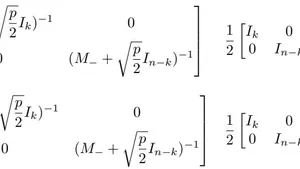
\[\times \left[ \begin{array}{c c} \frac {1}{2} \left[ \begin{array}{c c} (M _ {+} + \sqrt {\frac {p}{2}} I _ {k}) ^ {- 1} & 0 \\0 & (M _ {-} + \sqrt {\frac {p}{2}} I _ {n - k}) ^ {- 1} \end{array} \right] & \frac {1}{2} \left[ \begin{array}{c c} I _ {k} & 0 \\0 & I _ {n - k} \end{array} \right] \\- \frac {1}{2} \left[ \begin{array}{c c} (M _ {+} + \sqrt {\frac {p}{2}} I _ {k}) ^ {- 1} & 0 \\0 & (M _ {-} + \sqrt {\frac {p}{2}} I _ {n - k}) ^ {- 1} \end{array} \right] & \frac {1}{2} \left[ \begin{\array}{c c} I _ {k} & 0 \\0 & I _ {n - k} \end{array} \right] \end{array} \right] \left[ \begin{array}{c c} Q _ {d \tilde {b}} ^ {- 1} & 0 \\0 & Q _ {d \tilde {b}} ^ {- 1} \end{array} \right]\]
\[= \left[ \begin{array}{c c} Q _ {d \tilde {b}} & 0 \\0 & Q _ {d \tilde {b}} \end{array} \right] \left[ \begin{array}{c c} \frac {1}{2} \left[ \begin{array}{c c} I _ {k} & 0 \\0 & 0 \end{array} \right] & \frac {1}{2} \left[ \begin{array}{c c} M _ {+} + \sqrt {\frac {p}{2}} I _ {k} & 0 \\0 & 0 \end{array} \right] \\\frac {1}{2} \left[ \begin{array}{c c} (M _ {+} + \sqrt {\frac {p}{2}} I _ {k}) ^ {- 1} & 0 \\0 & 0 \end{array} \right] & \frac {1}{2} \left[ \begin{array}{c c} I _ {k} & 0 \\0 & 0 \end{array} \right] \end{array} \right] \left[ \begin{array}{c c} Q _ {d \tilde {b}} ^ {- 1} & 0 \\0 & Q _ {d \tilde {b}} ^ {- 1} \end{array} \right]\]
\[= \left[ \begin{array}{c c} Q _ {d \tilde {b}} \left[ \begin{array}{c c} \frac {1}{2} I _ {k} & 0 \\0 & 0 \end{array} \right] Q _ {d \tilde {b}} ^ {- 1} & Q _ {d b} \left[ \begin{array}{c c} \frac {1}{2} (M _ {+} + \sqrt {\frac {p}{2}} I _ {k}) & 0 \\0 & 0 \end{array} \right] Q _ {d \tilde {b}} ^ {- 1} \\Q _ {d \tilde {b}} \left[ \begin{array}{c c} \frac {1}{2} (M _ {+} + \sqrt {\frac {p}{2}} I _ {k}) ^ {- 1} & 0 \\0 & 0 \end{array} \right] Q _ {d \tilde {b}} ^ {- 1} & Q _ {d \tilde {b}} \left[ \begin{array}{c c} \frac {1}{2} I _ {k} & 0 \\0 & 0 \end{array} \right] Q _ {d \tilde {b}} ^ {- 1} \end{array} \right]\]
\[= \left[ \begin{array}{c c} \widetilde {\mathcal {P}} _ {1 1} ^ {(d)} & \widetilde {\mathcal {P}} _ {1 2} ^ {(d)} \\\widetilde {\mathcal {P}} _ {2 1} ^ {(d)} & \widetilde {\mathcal {P}} _ {2 2} ^ {(d)} \end{array} \right]\]
It follows that
\[\widetilde {\mathcal {P}} _ {1 1} ^ {(d)} = Q _ {d} \left[ \begin{array}{c c} \frac {1}{2} I _ {k} & 0 \\0 & 0 \end{array} \right] Q _ {d \tilde {b}} ^ {- 1} = \frac {1}{2} \widetilde {\mathbb {P}} _ {\infty}\]
\[\widetilde {\mathcal {P}} _ {1 2} ^ {(d)} = \frac {1}{2} Q _ {d \tilde {b}} \left[ \begin{array}{c c} M _ {+} + \sqrt {\frac {p}{2}} I _ {k} & 0 \\0 & 0 \end{array} \right] Q _ {d \tilde {b}} ^ {- 1}\]
\[\widetilde {\mathcal {P}} _ {2 1} ^ {(d)} = \frac {1}{2} Q _ {d b} \left[ \begin{array}{c c} (M _ {+} + \sqrt {\frac {p}{2}} I _ {k}) ^ {- 1} & 0 \\0 & 0 \end{array} \right] Q _ {d \tilde {b}} ^ {- 1}\]
\[\widetilde {\mathcal {P}} _ {2 2} ^ {(d)} = Q _ {d \tilde {b}} \left[ \begin{array}{c c} \frac {1}{2} I _ {k} & 0 \\0 & 0 \end{array} \right] Q _ {d \tilde {b}} ^ {- 1} = \frac {1}{2} \widetilde {\mathbb {P}} _ {\infty}\]
with we have
\[\begin{array}{l} A = A _ {d \tilde {b}} - \left(\frac {p}{2} - d - i p b\right) B \\= Q _ {d \tilde {b}} \left[ \begin{array}{c c} \left(M _ {+} + \sqrt {\frac {p}{2}} I _ {k}\right) ^ {2} - \left(\frac {p}{2} - d - i p \tilde {b}\right) B _ {1} & - \left(\frac {p}{2} - d - i p \tilde {b}\right) B _ {2} \\- \left(\frac {p}{2} - d - i p \tilde {b}\right) B _ {3} & \left(M _ {-} + \sqrt {\frac {p}{2}} I _ {n - k}\right) ^ {2} - \left(\frac {p}{2} - d - i p \tilde {b}\right) B _ {4} \end{array} \right] Q j _ {d \tilde {b}} ^ {- 1} \end{array}\]
where and
\[\begin{array}{r l} & {\widetilde {\mathbb {P}} _ {\infty} A = Q _ {d \tilde {b}} \left[ \begin{array}{c c} I _ {k} & 0 \\0 & 0 \end{array} \right] \left[ \begin{array}{c c} \left(M _ {+} + \sqrt {\frac {p}{2}} I _ {k}\right) ^ {2} - \left(\frac {p}{2} - d - i p \tilde {b}\right) B _ {1} & - \left(\frac {p}{2} - d - i p \tilde {b}\right) B _ {2} \\- \left(\frac {p}{2} - d - i p \tilde {b}\right) B _ {3} & \left(M _ {-} + \sqrt {\frac {p}{2}} I _ {n - k}\right) ^ {2} - \left(\frac {p}{2} - d - i p \tilde {b}\right) B _ {4} \end{array} \right] Q _ {d \tilde {b}} ^ {- 1}} \\& {\quad = Q _ {d b} \left[ \left( \begin{array}{c c} M _ {+} + \sqrt {\frac {p}{2}} I _ {k} \end{array} \right) ^ {2} - (\frac {p}{2} - d - i p \tilde {b}) B _ {1} \begin{array}{c c} 0 \\0 \end{array} \right] Q _ {d \tilde {b}} ^ {- 1}} \\& {\quad = 4 (\widetilde {\mathcal {P}} _ {1 2} ^ {(d)}) ^ {2} - (p - 2 d - 2 i p \tilde {b}) B \widetilde {\mathcal {P}} _ {1 1} ^ {(d \tilde {b})}} \end{array}\]
so (3.18) et (3.19).
Remark 3.1 We note that:
-
If the parameter , hence the equalities (3.19) are reduced to .
-
If the parameter , hence the equalities (3.19) are reduced to .
-
If the parameters , hence the equalities (3.19) are reduced to .
Algorithm 3.3 (DichoP)
being the projector on the right subspace of associated with the eigenvalues outside the parabola and the matrix whose norm gives the dichotomy criterion.
- If and , set
\[\mathcal {A} = \left( \begin{array}{c c} - \sqrt {\frac {p}{2}} B & A \\I _ {n} & - \sqrt {\frac {p}{2}} I _ {n} \end{array} \right) \quad a n d \quad \mathcal {B} = \left( \begin{array}{c c} B & 0 \\0 & I _ {n} \end{array} \right)\]
\[\mathcal {A} = \left( \begin{array}{c c} - \sqrt {\frac {p}{2}} B & A - i p b B \\I _ {n} & - \sqrt {\frac {p}{2}} I _ {n} \end{array} \right) \qquad a n d \quad \mathcal {B} = \left( \begin{array}{c c} B & 0 \\0 & I _ {n} \end{array} \right)\]
\[\mathcal {A} = \left( \begin{array}{c c} - \sqrt {\frac {p}{2}} B & A + (\frac {p}{2} - d) B \\I _ {n} & - \sqrt {\frac {p}{2}} I _ {n} \end{array} \right) \qquad a n d \quad \mathcal {B} = \left( \begin{array}{c c} B & 0 \\0 & I _ {n} \end{array} \right)\]
\[\mathcal {A} = \left( \begin{array}{c c} - \sqrt {\frac {p}{2}} B & A + (\frac {p}{2} - d - i p \tilde {b}) B \\I _ {n} & - \sqrt {\frac {p}{2}} I _ {n} \end{array} \right) \qquad a n d \quad \mathcal {B} = \left( \begin{array}{c c} B & 0 \\0 & I _ {n} \end{array} \right)\]
-
Using Algorithm 2.3 to , compute the Projector onto the right eigenspace of associated with the eigenvalues on the right half-plane of the complex plane and the matrix ;
-
If is not large, determine the projectors by
\[\mathbb {P} = 2 \widetilde {\mathcal {P}} _ {1}\]
IV. NUMERICAL TESTS
Example 4.1 We consider the matrix pencil of order 20 defined by [18]
\[A = \left\{ \begin{array}{c c c} a _ {2 i, 2 i} = - \frac {1}{3} & \text{if} & 1 \leq i \leq 10 \\ a _ {2 i - 1, 2 i + 1} = 1 & \text{if} & 1 \leq i \leq 9 \\ a _ {2 i + 1, 2 i - 1} = \frac {1}{3} & \text{if} & 1 \leq i \leq 9 \\ a _ {2 i, 2 i + 1} = 3 & \text{if} & 1 \leq i \leq 9 \\ a _ {i, j} = 0 & & \text{otherwise} \end{array} \right. \quad \text{and} \quad B = \left\{ \begin{array}{c c c} b _ {2 i - 1, 2 i - 1} = - \frac {1}{4} & \text{if} & 1 \leq i \leq 10 \\ b _ {2 i, 2 i + 2} = - 1 & \text{if} & 1 \leq i \leq 9 \\ b _ {2 i + 2, 2 i} = 5 & \text{if} & 1 \leq i \leq 9 \\ b _ {2 i, 2 i - 1} = 2 & \text{if} & 1 \leq i \leq 9 \\ b _ {i, j} = 0 & & \text{otherwise} \end{array} \right.\tag{4.1}\]
{"image_source":{"path":"images/c807bab1e84bfc41cffd5145396d5b83134f08f80275867db2fbf8d7cd2830b2.jpg"},"content":"","chart_caption":[],"chart_footnote":[]} {"image_source":{"path":"images/85cc1a37098f69d9ea392059a84322154bc113251b77c433dfabb1fd113e327e.jpg"},"content":"","chart_caption":[],"chart_footnote":[]}
{"image_source":{"path":"images/5f78c4d0b59542b2026f2f5d47e3d64af762ff26fb65755a5be52a14b50f2aab.jpg"},"content":"","chart_caption":[],"chart_footnote":[]} {"image_source":{"path":"images/eee51e851a26251b152476bcba56715bc812f68c88119ec3e922eb1b84bd95cd.jpg"},"content":"","chart_caption":[{"type":"text","content":"Figure 1: Partition of the spectrum of the matrix pencil "},{"type":"equation_inline","content":"zB - A"},{"type":"text","content":" by the off-center circle with center with affix "},{"type":"equation_inline","content":"z0"},{"type":"text","content":"."}],"chart_footnote":[]}
Table 1: Traces, norms and quality of the spectral projector by applying Algorithm 3.1 for four values of the couple
| (b,r) | tr(P0) | ||P0|| | ||P20-P0|| | ||P0W-WP0|| | ||H0|| |
| (2,3) | 16 | 1.9428 1004 | 4.4207 10-10 | 4.9178 10-7 | 6.5654 1010 |
| (3i,1.5) | 0 | 0 | 0 | 0 | 4.2800 1008 |
| (0,3.5) | 16 | 1.9089 104 | 1.5983 10-11 | 4.6416 10-6 | 6.6210 1010 |
| (2-2i,3) | 13 | 2.1814 104 | 5.3396 10-9 | 3.3987 10-7 | 8.8018 1010 |
Table 2: Traces, norms and quality of the spectral projector
by applying Algorithm 3.2 for values
| (a,b,z0) | tr(P∞) | ||P∞|| | ||P2∞-P∞|| | ||P∞W-WP∞|| | ||H∞|| |
| (6,√(3),1) | 20 | 1 | 7.7410 10-14 | 2.8899 10-12 | 1.3900 108 |
| (2,√(2),i) | 11 | 2.3358 104 | 1.5964 10-7 | 1.0407 10-6 | 5.0865 1010 |
| (4,1,1-i) | 5 | 1.6850 104 | 5.4046 10-7 | 2.8924 10-6 | 3.9620 1011 |
| (3,1.2,2+2i) | 0 | 3.0725 10-8 | 3.0725 10-8 | 1.4260 10-7 | 1.9655 109 |
Table 3: Traces, norms and quality of the spectral projectorP by applying Algorithm 3.3 for four values p, b and d.
| $(p,b,d)$ | $tr(\mathbb{P})$ | $\|\mathbb{P}\|$ | $\|\mathbb{P}^{2}-\mathbb{P}\|$ | $\|\mathbb{P}W-W\mathbb{P}\|$ | $\|\mathbb{H}\|$ |
| $(2,0,10)$ | 20 | 1 | $4.8955\ 10^{-13}$ | $1.0086\ 10^{-12}$ | $4.2198\ 10^{6}$ |
| $(1.5,3,1)$ | 16 | $2.7889\ 10^{-8}$ | $2.7889\ 10^{-8}$ | $2.0312\ 10^{-8}$ | $1.7304\ 10^{10}$ |
| $(1,4,1)$ | 0 | $3.5172\ 10^{-9}$ | $3.5172\ 10^{-9}$ | $2.6957\ 10^{-8}$ | $3.5087\ 10^{8}$ |
| $(3,2,3)$ | 3 | $1.8947\ 10^{4}$ | $1.4058\ 10^{-7}$ | $1.3711\ 10^{-7}$ | $9.0937\ 10^{11}$ |
{"image_source":{"path":"images/5679fab429fc35ba083b00f7ce1f394a44991d227eb887ec943397c5590ccbba.jpg"},"content":"","chart_caption":[],"chart_footnote":[]} {"image_source":{"path":"images/6bb9917572771736bcb80aad6b4b101528def57fc06ef1193aaeb16f15084acb.jpg"},"content":"","chart_caption":[],"chart_footnote":[]}
{"image_source":{"path":"images/d4f36267d40082f9eaee39e9b56a72aa847b0f367d950a23ab6e77dff392acf2.jpg"},"content":"","chart_caption":[],"chart_footnote":[]} {"image_source":{"path":"images/80401b1b6ad73d7153b634a0f97e3eb5cef0d3a8871f58045f8db024386f8a23.jpg"},"content":"","chart_caption":[],"chart_footnote":[]}
{"image_source":{"path":"images/c8c7985c2814ffae3b4178487eb999ca6071ae7723a0a7a6934fafd4c2dcc332.jpg"},"content":"","chart_caption":[{"type":"text","content":"Figure 2: Partition of the spectrum of the matrix pencil "},{"type":"equation_inline","content":"zB - A"},{"type":"text","content":" by the off-center ellipse with center with affix "},{"type":"equation_inline","content":"z0"},{"type":"text","content":" and parameters "},{"type":"equation_inline","content":"a"},{"type":"text","content":" and "},{"type":"equation_inline","content":"b"},{"type":"text","content":"."}],"chart_footnote":[]} {"image_source":{"path":"images/5dd013cb0c3179214308832334b168ad86b2f312524c969634902ec7deb1c228.jpg"},"content":"","chart_caption":[],"chart_footnote":[]}
{"image_source":{"path":"images/0e37f1de046ea9c2022d1edbe5510d5b67c126f5bb42500f3bde94a084c29908.jpg"},"content":"","chart_caption":[],"chart_footnote":[]} {"image_source":{"path":"images/2dab88631c36e73ec197955bcaad0fffcc98adc4f8aae8e78ebca2834f0b23d8.jpg"},"content":"","chart_caption":[{"type":"text","content":"Figure 3: Partition of the spectrum of the matrix pencil "},{"type":"equation_inline","content":"zB - A"},{"type":"text","content":" by the parabola of equation "},{"type":"equation_inline","content":"2p(d - x) = y^2"},{"type":"text","content":"."}],"chart_footnote":[]}
The graphs above effectively show a dichotomy of the spectrum of the matrix pencil by the various curves which are the circle, the ellipse and the parabola all not centered at the origin. To corroborate our algorithms, we give in tables, the values of the norms of the projector P and of the norm of the dichotomy matrix H.
We note that the values taken by the norms of the projector and of its dichotomy criterion are high. This is due to the fact that the matrices and are badly conditioned ( et where ).
Example 4.2 Consider the matrices
\[A = \left[ \begin{array}{r r r r r r} 0. 4 9 & 0. 8 9 & 0. 3 3 & 0. 3 2 & 1. 0 9 & - 0. 0 1 \\1. 0 3 & - 1. 1 5 & - 0. 7 5 & 0. 3 1 & 1. 1 1 & 1. 5 3 \\0. 7 3 & - 1. 0 7 & 1. 3 7 & - 0. 8 6 & - 0. 8 6 & - 0. 7 7 \\- 0. 3 0 & - 0. 8 1 & - 1. 7 1 & - 0. 0 3 & 0. 0 8 & 0. 3 7 \\0. 2 9 & - 2. 9 4 & - 0. 1 0 & - 0. 1 6 & - 1. 2 1 & - 0. 2 3 \\- 0. 7 9 & 1. 4 4 & - 0. 2 4 & 0. 6 3 & - 1. 1 1 & 1. 1 2 \end{array} \right], \quad B = \left[ \begin{array}{r r r r r r} 5 & 1. 5 & 0 & 0 & 1 & 0 \\0 & 4 & 1 & 1 & 0 & 1 \\0 & 1 & 3 & 1 & 0 & 0 \\1 & 0 & 0 & 2 & 1 & 1 \\1 & 1 & 0 & 0 & 2 & 1 \\1 & 0 & 0 & 0 & 0 & 1 \end{array} \right]\tag{4.2}\]
with matrix B a no singular matrix.
{"image_source":{"path":"images/e184291c68d1b8f575340086887229f4c47d49d5acaaf6991f648ef4540285f5.jpg"},"content":"","chart_caption":[],"chart_footnote":[]} {"image_source":{"path":"images/046c43dbc5fffe053d04c4d80d6ca0ad81cb99bbfcc6f11087392b4427b2f8d7.jpg"},"content":"","chart_caption":[],"chart_footnote":[]}
{"image_source":{"path":"images/9f8da8ceee96eb8b49a6ffaf31beded84e3bbb1c2d751df9805b0bf91d27037d.jpg"},"content":"","chart_caption":[],"chart_footnote":[]} {"image_source":{"path":"images/e87537a9359d8c338d7c46603a4cd626d356d6cafeaec7ea12874a63bc67a283.jpg"},"content":"","chart_caption":[{"type":"text","content":"Figure 4: Partition of the spectrum of the matrix pencil "},{"type":"equation_inline","content":"zB - A"},{"type":"text","content":" by the off-center circle with center with affix "},{"type":"equation_inline","content":"z0"},{"type":"text","content":"."}],"chart_footnote":[]}
Table 4: Traces, norms and quality of the spectral projector by applying Algorithm 3.1 for four values of the couple
| (b,r) | tr(P0) | ||P0|| | ||P20-P0|| | ||P0W-WP0|| | ||H0|| |
| (2,4) | 6 | 1 | 3.1317 10-16 | 4.4730 10-16 | 1.3256 |
| (3i,1.5) | 0 | 0 | 0 | 0 | 0.4696 |
| (0,3.5) | 6 | 1 | 3.4282 10-16 | 7.9911 10-16 | 1.2442 |
| (2+2i,3) | 4 | 1.8397 | 5.8237 10-16 | 4.3141 10-15 | 68.5791 |
{"image_source":{"path":"images/4fb0a7cde79991d58a0cbd5d11c3e7871539c0955e4d4e87a09bbb5ee15092f9.jpg"},"content":"","chart_caption":[{"type":"text","content":"Figure 5: Partition of the spectrum of the matrix pencil "},{"type":"equation_inline","content":"zB - A"},{"type":"text","content":" by the off-center ellipse with center with affix "},{"type":"equation_inline","content":"z0"},{"type":"text","content":" and parameters "},{"type":"equation_inline","content":"a"},{"type":"text","content":" and "},{"type":"equation_inline","content":"b"},{"type":"text","content":"."}],"chart_footnote":[]}
Table 5: Traces, norms and quality of the spectral projector by applying Algorithm 3.2 for values .
| (a,b,z0) | tr(P∞) | ||P∞|| | ||P2∞-P∞|| | ||P∞W-WP∞|| | ||H∞|| |
| (6,√(3),1) | 6 | 1 | 6.6926 10-16 | 8.9554 10-16 | 0.1147 |
| (2,√(2),i) | 5 | 1.7637 | 8.2272 10-16 | 8.3327 10-15 | 17.3309 |
| (4,1,1-1.5i) | 1 | 1.7637 | 1.1051 10-15 | 8.9629e-15 10-15 | 0.3607 |
| (3,1.2,2+2i) | 0 | 1.8846 10-15 | 1.8846 10-15 | 3.9832 10-15 | 0.3056 |
{"image_source":{"path":"images/8a8abe1043987d5bfe166856306899c07bd26af27569c2f7f7c4b373b7f1ac60.jpg"},"content":"","chart_caption":[{"type":"text","content":"Figure 6: Partition of the spectrum of the matrix pencil "},{"type":"equation_inline","content":"zB - A"},{"type":"text","content":" by the parabola of equation "},{"type":"equation_inline","content":"2p(d - x) = y^2"},{"type":"text","content":"."}],"chart_footnote":[]}
Table 6: Traces, norms and quality of the spectral projector P by applying Algorithm 3.3 for four values p, b and d.
| $(p,b,d)$ | $tr(\mathbb{P})$ | $\|\mathbb{P}\|$ | $\|\mathbb{P}^{2}-\mathbb{P}\|$ | $\|\mathbb{P}W-W\mathbb{P}\|$ | $\|\mathbb{H}\|$ |
| (2,0,10) | 6 | 1 | $4.5305e-16\ 10^{-16}$ | $3.9732\ 10^{-16}$ | 1.4152 |
| (1.5,3,1) | 0 | $5.0943\ 10^{-15}$ | $5.0943\ 10^{-15}$ | $4.8198\ 10^{-15}$ | 1.3944 |
| (1,4,1) | 0 | 0 | $2.6692\ 10^{-15}$ | $6.6636\ 10^{-15}$ | 1.2688 |
| (3,2,3) | 0 | $5.5735\ 10^{-15}$ | $5.5735\ 10^{-15}$ | $8.3372\ 10^{-15}$ | 8.7003 |
The graphs above effectively show a dichotomy of the spectrum of the matrix pencil by the various curves which are the circle, the ellipse and the parabola all not centered at the origin. To corroborate our algorithms, we give in tables, the values of the norms of the projector P and of the norm of the dichotomy matrix H.
We can notice that the values of the norm of are small. This proves the very good quality of the dichotomy carried out
V. CONCLUSION
After a few reminders on methods of spectral dichotomy of a pencil matrix with respect to a circle, an ellipse or a parabola all not centered at the origin and/or not symmetrical with respect to the abscissa axis, we presented, by making changes of variables, methods of spectral dichotomy of a pencil matrix with respect to an off-center circle, an off-center ellipse or any parabola. In the spectral dichotomy method of a pencil matrix with respect to
-
a circle , not originally centered, by considering the change of variable , we obtain projector on the invariant space of the pencil matrix corresponding to the eigenvalues inside the circle and a Matrix whose the norm indicates the quality of the projector, by applying the spectral dichotomy method of the pencil matrix with respect to the circle centered at the origin.
-
an ellipse centered at a point , by considering the change of variable , we obtain the projector on the right invariant space of corresponding to the eigenvalues outside the ellipse and a Matrix whose the norm indicates the quality of the projector, by applying the spectral dichotomy method of a pencil matrix with respect to the ellipse centered at the origin.
-
any parabola of equation with , by considering the change of variable , we obtain on the right subspace of associated with the eigenvalues outside the parabola and a Matrix whose the norm indicates the quality of the projector, by applying the spectral dichotomy method of a pencil matrix with respect to the parabola studied by Malyshev and Sadkane.
Numerical tests on two examples of matrices pencils show that the presented methods compute well the projectors if there are no eigenvalues on or in a close neighborhood of the figures.