


IntelliPaper
Abstract
This research examines the impact of Gross Domestic Product (GDP) on CO2 emissions in four well-developed Asian countries—South Korea, Singapore, Taiwan, and Hong Kong—over the period from 1960 to 2019. To analyze the relationships, regression was performed using the Generalized Least Squares (GLS) method in STATA-14. The results indicate that all regressors are significant, and to address the issue of autocorrelation in the model, an Autoregressive Lag model was used. By adding the lag of an independent variable to the model, the problem of autocorrelation was resolved. Consequently, the model's goodness-of-fit improved, and the significance levels of the regressors were confirmed. Based on the research findings, it can be concluded that the economic growth of these countries leads to an increase in carbon dioxide emissions into the external environment.
Explore Digital Article Text
I. INTRODUCTION.
The reason we chose this specific topic is that today, the issue of environmental pollution, particularly the problem of carbon dioxide emissions that have a range of negative and harmful effects on living organisms, is becoming one of the most pressing concerns. For the analysis, four countries from Asia, specifically the
Asian Tiger countries, were selected. These countries have both developed and developing economies, and the analyses conducted can also be applied to Uzbekistan.
The aim of the research presented in the monograph is to evaluate the impact of economic and environmental policies on the state of the environment and to develop methods for this assessment. To achieve this goal, the following tasks were addressed:
Developing the proposed approach, improving the previously established ones, and creating new mathematical models and methods based on the identified connections between economic and environmental indicators that will allow for the assessment of the impact of various factors on environmental pollution.
The country analysis demonstrates the relationship between GDP growth and CO2 emissions in the Asian Tiger countries.
Based on the constructed pollution functions, conducting a comparative analysis of the impact of economic development on the environment in these countries and neighboring countries (regions) with similar natural-climatic conditions and similar economic structures.
Since the works of J. Forrester, M. Mesarovich, and E. Pestel, significant attention has been given to the environmental consequences of economic development. Since the late 1980s, ecological economics has developed rapidly, including the development of specialized mathematical models.
Among the modern studies in the field of ecological and economic interactions are the works of T. A. Akimova, S. N. Bobylev, I. P. Glazyrina, A. A. Gusev, V.
I. Danilov-Danilyan, M.
F. Zamyatina, G. E. Mekush, N.
V. Pakhomova, I.
V. Sheravniy, R. I., R. I., and others. Special models are developed to assess the interaction of economic and ecological processes, which together describe the behavior of ecological and economic systems and allow for the identification and quantitative assessment of the main factors influencing changes in the ecological situation.
At the same time, the impact of significant factors within a single year and their effect on the environment, as well as their influence on indicators in subsequent years, has not been sufficiently studied.
II. METHODOLOGY
Figure 1: Digital Descriptive Statistics
| Variable | Obs | Mean | Std. Dev. | Min | Max |
| GDP | 239 | 9.64e+11 | 2.33e+12 | 5.95e+09 | 1.43e+13 |
| CO2 | 237 | 997993.3 | 2249859 | 674.728 | 1.07e+07 |
In the STATA-14 program, the "sum" command is used to view the number of observations, the arithmetic mean, the quadratic mean deviation, as well as the minimum and maximum values.
{"image_source":{"path":"images/016f0fbf979f4635e8c198101de1e1fe2d7c6fd6d9fc3d11dd1b4f22c9cf8be7.jpg"},"content":"","chart_caption":[],"chart_footnote":[]} {"image_source":{"path":"images/8ef1af0708544fac4d9241285c820b7056cd11f76e9b9400b88af3b3883f1b37.jpg"},"content":"","chart_caption":[{"type":"text","content":"Figures 2-3: Normal Distribution Analysis"}],"chart_footnote":[]}
The comparison between statistical indicators and the normal distribution is illustrated in Figures 2-3, where we can observe that our indicators closely approximate the normal distribution.
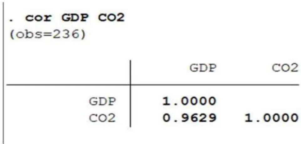
{"image_source":{"path":"images/64ff11f4d6566dd3d9fd833d6cb7ee38e17e14c867e7bf84da2d73c27b3628ab.jpg"},"content":"","chart_caption":[{"type":"text","content":"The results of the correlation analysis show that GDP and CO2 have a strong positive correlation."},{"type":"text","content":"Figure 5"}],"chart_footnote":[]}
The analysis of carbon dioxide emission indicators by country is presented in Figure 5. Although the patterns may appear different at various scales, the scatter plots of the countries present nearly the same shape.
III. ANALYSIS OF RESULTS
The results of the regression analysis on the collected data are presented in Figure 6.
Figure 6
| Source | SS | df | MS | Number of obs = 236 | |
| F(1, 234) = 2981.70 | |||||
| Model | 1.1068e+15 | 1 | 1.1068e+15 | Prob > F = 0.0000 | |
| Residual | 8.6856e+13 | 234 | 3.7118e+11 | R-squared = 0.9272 | |
| Adj R-squared = 0.9269 | |||||
| Total | 1.1936e+15 | 235 | 5.0792e+12 | Root MSE = 6.1e+05 | |
| CO2 | Coef. | Std. Err. | t | P>|t| | [95% Conf. Interval] |
| GDP | 9.28e-07 | 1.70e-08 | 54.60 | 0.000 | 8.94e-07 |
| _cons | 100177.3 | 42961.42 | 2.33 | 0.021 | 15536.67 |
The results of our regression analysis show that a 1% increase in GDP leads to a 9.28% increase in CO2 emissions. The overall coefficient of determination is 92.72%. Our p-value indicates that the result is statistically significant.
It is necessary to check the regression results according to the Gauss-Markov conditions. The results are presented in Figures 7 and 8.
{"code_caption":[],"code_content":[{"type":"text","content":". estat hettest\nBreusch-Pagan/Cook-Weisberg test for heteroskedasticity\nHo: Constant variance\nVariables: fitted values of co2\nchi2(1) = 0.04\nProb > chi2 = 0.8477"}],"code_language":"txt"}
Figure 7
Breusch-Godfrey LM test for autocorrelation
Figure 8
| lags (p) | chi2 | df | Prob > chi2 |
| 1 | 221.918 | 1 | 0.0000 |
| 2 | 221.934 | 2 | 0.0000 |
| 3 | 222.055 | 3 | 0.0000 |
| 4 | 222.082 | 4 | 0.0000 |
| 5 | 222.355 | 5 | 0.0000 |
The Breusch-Pagan heteroscedasticity test is presented in Figure 7. According to its results, there is no heteroscedasticity problem in our model. The Breusch-Godfrey test, presented in
Figure 8, checks the model for autocorrelation issues. The test results show that autocorrelation exists even at the 5th-order lag. Although we do not present it here, we also checked that autocorrelation causes issues at all existing lags.
To address the autocorrelation issue in the model, we use an Autoregressive Lag model. By adding the lag of the independent variable to the model, we resolve the autocorrelation problem in the model.
The results of the Autoregressive Lag model are presented in Figure 9. According to these results, the model's coefficient of determination has improved, and the significance levels of the regressors have been confirmed. A increase in GDP leads to a increase in carbon dioxide emissions.
Figure 9: The results of our research confirmed the views presented in the scientific literature.
| Source | SS | df | MS | Number of obs = 234 | |
| F(2, 231) = 3216.27 | |||||
| Model | 1063.53541 | 2 | 531.767705 | Prob > F = 0.0000 | |
| Residual | 38.1927923 | 231 | .165336763 | R-squared = 0.9653 | |
| Total | 1101.7282 | 233 | 4.72844722 | Adj R-squared = 0.9650 | |
| Root MSE =.40662 | |||||
| co2 | Coef. | Std. Err. | t | P>|t| | [95% Conf. Interval] |
| gdp | .2099356 | .0348614 | 6.02 | 0.000 | .1412487.2786225 |
| co2 | |||||
| L1. | .8302775 | .0276643 | 30.01 | 0.000 | .775771.8847841 |
| _cons | -3.463209 | .6361157 | -5.44 | 0.000 | -4.716539 -2.209879 |
IV. CONCLUSION
Based on the conducted research, it can be concluded that the economic growth of countries leads to an increase in carbon dioxide emissions into the external environment. This phenomenon negatively impacts the environment, causes ecological degradation, and leads to the formation of ozone holes. Therefore, this process should be monitored by governments to maintain a balance.
Conflict of Interest
The authors declare no conflict of interest.
Ethical Approval
Not applicable
Data Availability
The datasets used in this study are openly available at [repository link] and the source code is available on GitHub at [GitHub link].
Funding
This work did not receive any external funding.
References
Cite this article
Related Research


Special Issue
Launch a focused special issue to highlight research, emerging trends, and expert insights in your academic field.