


Abstract
In this article, we present a new quantification method to realize the principal component analysis (PCA) for symbolic data tables. We first describe the nesting property for the monotone point sequences and the correlation matrix by the rank correlation coefficient. Then, we present the object splitting method by which interval valued data table can be transformed to a usual numerical data table. We are able to apply the traditional PCA to this transformed data table. The quantile method is a generalization of the object splitting method, and can manipulate histograms, nominal multi-value types, and other types simultaneously. We present several experimental results in order to illustrate the usefulness of the quantile method. 2011 Wiley Periodicals, Inc. Statistical Analysis and Data Mining 4: 184–198, 2011
Explore Digital Article Text
I. INTRODUCTION
The generalization of the principal component analysis (PCA) is an important research theme in the symbolic data analysis . The main purpose of the traditional PCA is to transform a number of possibly correlated variables into a small number of uncorrelated variables called principal components. Chouakria proposed the extension of the PCA to interval data as vertices principal component analysis (V-PCA). Chouakria et al. proposed also the centers method of PCA (C-PCA) for interval data, and they presented a comparative example for the V-PCA and the C-PCA. Lauro and Palumbo proposed symbolic object principal component analysis (SO-PCA) as an extended PCA to any numerical data structure. Lauro et al. summarize various methods of SO-PCA for interval data. The author also proposed a general "Symbolic PCA" (S-PCA) based on the quantification method by using the generalized Minkowski metrics . In this approach, we first transform the given symbolic data table to a usual numerical data table, and then we execute the traditional PCA on the transformed data table.
In this article, another quantification method for symbolic data tables based on the monotone structures of objects is presented. In Section 2, first we describe the case of point sequences in a d-dimensional Euclidean space. The monotone structures are characterized by the nesting of the Cartesian join regions associated with pairs of objects. If the given point sequence is monotone in the Euclidean d space, the property is also satisfied in any feature axis. In other words, a nesting structure of the given point sequence in the d space confines the orders of points in each feature axis to be similar. Therefore, we can evaluate the degree of similarity between features based on the Kendall or the Spearman's rank correlation coefficients. Then, we can execute a traditional PCA based on the correlation matrix by the selected rank correlation coefficient. Secondly, we describe the "object splitting method" for SO-PCA for interval-valued data . This method splits each of N symbolic objects described by d interval-valued features into the two d-dimensional vertices called the "minimum sub-object" and the "maximum sub object". We should point out the fact that any interval object can be reproduced from the minimum and the maximum sub-objects. Moreover, the nesting structure of interval objects in the d space confines the orders of the minimum and the maximum sub-objects in each feature axis to be similar. Therefore, we can evaluate again the degree of similarity between features based on the Kendall or the Spearman's rank correlation coefficients on the standard numerical data table. We can execute a traditional PCA based on the correlation matrix by the selected rank correlation coefficient. As a further extension to manipulate histogram data, nominal multi-valued data, and others, we describe the "quantile method" for S-PCA [12] in Section 4.
The problem is how to obtain a common numerical representation of objects described by mixed types of features. For example, in histogram data, the numbers of subinter vals (bins) of the given histograms are mutually different in general. Therefore, we first define the cumulative distribution function for each histogram. Then, we select a common integer number m to generate the "quantiles" for all histograms. As the result, for each histogram, we have an -tuple composed of quantiles and the minimum and the maximum values of the whole interval of the histogram. Then, we split each object into sub-objects: the minimum sub-object, quantile sub objects and the maximum sub-object. By virtue of the monotonic property of the distribution function, sub-objects of an object satisfy automatically a nesting structure. Therefore, the nesting of N objects described by the minimum and the maximum sub-objects in the d space confines the orders of sub-objects in each feature axis to be similar. Again, we can evaluate the degree of similarity between features by the Kendall or the Spearman's rank correlation coefficient, and then execute a traditional PCA.
Interval-valued data may be regarded as a special histogram-valued data, where only one bin organizes the histogram. Furthermore, we can also split nominal multi-valued data into sub-objects based on the distribution function associated with rank values attached to categorical values of an object. Therefore, by the quantile method we can transform a given general symbolic data table to an standard numerical data table, and then we can execute a traditional PCA on the transformed data table. In Section 5, we describe several experimental results in order to show the effectiveness of the quantile method. Section 6 is a summary.
II. MONOTONE STRUCTURES AND OBJECT SPLITTING METHOD
In this section, we describe some properties of monotone structures for point sequence and for interval objects. Then, we describe the object splitting method for S-PCA.
2.1. Monotone Structures for Point Sequence
Let a set of N objects U be represented by . Let each object be described by d numerical features, i.e. a vector in a d-dimensional Euclidean space .
DEFINITION 1: Rectangular region spanned by and .
Let be a rectangular region in spanned by the vectors and , and be defined by the following Cartesian product of d closed intervals.
where and are the operators to take the minimum value and the maximum value from a and b, respectively.
(b) Monotone decreasing.
In the following, we call as the Cartesian join (region) of objects and .
DEFINITION 2: Nesting structure
If a series of objects , ,..., satisfies the nesting property
the series is called a "nesting structure with the starting point and the ending point ".
In Fig. 1, (a) is a monotone increasing series, and (b) is a monotone decreasing series of objects. It should be noted that the two series of objects show the same nesting structures with starting point and ending point .
PROPOSITION 1: If a series of objects is a nesting structure with the starting point and the ending point in the space , the series satisfies the same structure in each feature (axis) of the space .
Proof: From the definition of rectangular region as in Eq. (1), we have
and
186 Statistical Analysis and Data Mining, Vol. 4 (2011) {"image_source":{"path":"images/41137a1fdbe4c18c3489d5c1e6ce082b9507144a96551790b192d3d3ab1ecac6.jpg"},"content":"","chart_caption":[{"type":"text","content":"(a) Monotone increasing."}],"chart_footnote":[]}
{"image_source":{"path":"images/3f16846068bb440353b1528ffa525510300bbb5ee9a0d2d9fd6cbd1c74f84747.jpg"},"content":"","chart_caption":[{"type":"text","content":"Fig. 1: Monotone structures of point sequence."}],"chart_footnote":[]}
Therefore, the relations of the Cartesian join regions , in Definition 2, require the following relations for each feature, i.e. for each ,
Although, there exist several ways to define the mono tone sequences of objects, i.e. monotone structures, we use the following definition.
DEFINITION 3: Monotone structure of a series of points.
A series of objects is called a monotone structure, if the series satisfies the nesting structure of Definition 2.
Since, for a pair of features, we can evaluate the degree of similarity between two sets of orders of objects for the same object set by using the Kendall or the Spearman's rank correlation coefficient, we have Proposition 2.
PROPOSITION 2: Correlation matrix S.
If a series of objects is a monotone structure in the space , the absolute value of each off diagonal element of the correlation matrix takes the maximum value one in the sense of the Kendall or the Spearman's rank correlation coefficient.
Proof: From Definition 3, any monotone structure must satisfy the nesting property of Definition 2. Then, from Proposition 1, the given series of objects has the identical nesting structure for each feature. This property exactly restricts the order of objects for each feature to be the same way or the reverse way according to the series of objects is monotone increasing or monotone decreasing. Therefore, if a series of objects is a monotone structure in , the absolute value of the correlation coefficient for each pair of features takes the maximum value one in the sense of the Kendall or the Spearman's rank correlation coefficient.
From Proposition 2, if many off-diagonal elements of S take highly correlated values, we can expect the existence of a large eigenvalue of S, and that the corresponding eigenvector reproduces well the original nesting property of the set of objects in the space .
EXAMPLE 1: As an intuitive example, suppose that the given set of objects in organizes an approximate monotone structure which is monotone increasing along each of d features, and the degrees of similarity between two features are the same for all possible pairs. Therefore, all off-diagonal elements of S take an identical value , . Then, it is known [14] that d eigenvalues of S become
and the eigenvector for is
Therefore, the given monotone structure of objects in is approximately reproduced around the eigenvector . As a particular case, when , the given set of objects organizes a complete monotone structure in the space . Then, the eigenvalue becomes d, i.e. its contribution ratio is 100%, and the order of the given object sequence in the space is exactly reproduced on the eigenvector .
In the above, we characterized monotone structures by the nesting property, and obtain the correlation matrix . The monotone structures include any linear structure as a special case. On the other hand, a monotone structure may be approximated well by an appropriately selected linear structure. This suggests that we can use also the Pearson correlation coefficient to evaluate the degree of similarity between two features instead of the Kendall and the Spearman's rank correlation coefficients.
2.2. Monotone Structures for Interval Objects
Let each object be described by d interval-valued features. Then, an object becomes a hyper rectangle in , i.e. the Cartesian product of d closed intervals:
where each interval is given by
Then, we can define the minimum vertex and the maximum vertex by
DEFINITION 4: The minimum sub-object and the max imum sub-object
Let the minimum vertex and the maximum vertex for each object be called the minimum sub object and the maximum sub-object, and be denoted by and , respectively.
EXAMPLE 2: In Table 1, the minimum and the maxi mum sub-objects of Linseed oil under the first four inter val features are represented by the vertices and , respectively.
PROPOSITION 3: From Definition 1, any interval object is represented in the space by the Cartesian join region .
Proof: From Eq. (1) in Definition 1 and (8–10), we see that
From Eq. (8), d respective intervals for and are
Thus the closed interval generated from two intervals and becomes
DEFINITION 5: We define the Cartesian join region based on Eq. (12) by
In this definition, we should note that, for each k, is equivalent to . Furthermore,
| Object | Specific gravity (g/cm3), | Freezing point (°C), | Iodine value, | Saponification value, | Major acids, |
| 1. Linseed | 0.930–0.935 | -27 to -18 | 170–204 | 118–196 | L, Ln, O, P, M |
| 2. Perilla | 0.930–0.937 | -5 to -4 | 192–208 | 188–197 | L, Ln, O, P, S |
| 3. Cotton | 0.916–0.918 | -6 to -1 | 99–113 | 189–198 | L, O, P, M, S |
| 4. Sesame | 0.920–0.926 | -6 to -4 | 104–116 | 187–193 | L, O, P, S, A |
| 5. Camellia | 0.916–0.917 | -21 to -15 | 80–82 | 189–193 | L, O |
| 6. Olive | 0.914–0.919 | 0–6 | 79–90 | 187–196 | L, O, P, S |
| 7. Beef | 0.860–0.870 | 30–38 | 40–48 | 190–199 | O, P, M, S, C |
| 8. Hog | 0.858–0.864 | 22–32 | 53–77 | 190–202 | L, O, P, M, S, Lu |
linoleic acid, linolenic acid, oleic acid, palmitic acid, myristic acid, searic acid, arachic acid, capric acid, lauric acid.
and are reduced to the minimum vertex and the maximum vertex in Eq. (10), respectively.
DEFINITION 6: Nesting structure for interval objects If a series of interval objects satisfies the nesting property
the series is called a "nesting structure with the starting object and the ending object ".
Fig. 2 shows a series of five interval objects. It should be noted that the nesting order of objects in each feature axis is the same as that in the two-dimensional space.
PROPOSITION 4: If a series of interval objects is a nesting structure with the starting object and the ending object in the space , the series has the same nesting in each feature (axis) of the space .
Proof: From the definition of the Cartesian join region as seen in Eq. (13), we have
{"image_source":{"path":"images/fbd73eecd40f2bc888c0a8961e9be9155655ef4de7a2b691941a2a01ce989224.jpg"},"content":"","chart_caption":[{"type":"text","content":"Fig. 2: A monotone structure of interval objects."}],"chart_footnote":[]} and
Therefore, the relations of the Cartesian join regions , in Definition 5, require the following relations for each feature, i.e. for each ,
We define the monotone structure of interval objects by the same way in Definition 3.
DEFINITION 7: Monotone structure of a series of interval objects.
A series of interval objects is called a monotone structure, if the series satisfies a nesting structure in Definition 6.
According to Definition 7, we assume a series of interval objects is a monotone structure in the space . Then, from Proposition 4, the series of objects satisfies the same nesting in each feature axis. However, the nesting in (17) is based on the closed intervals generated from two objects. Therefore, we cannot evaluate the degree of similarity between two features by direct use of the Kendall or the Spearman's rank correlation coefficient. To remove this difficulty, we split each interval object into the minimum sub-object and the maximum sub-object.
PROPOSITION 5: Monotone conditions by sub-objects. Let a series of interval objects be monotone in the space . Then, at least one condition of the following must be satisfied.
(1) The series of the minimum sub-objects, , ,..., , is monotone in .
(2) The series of the maximum sub-objects, , ,..., , is monotone in .
Proof: Assume that the conditions (1) and (2) are negated simultaneously. Then, there exists a nesting order k in which the object satisfies the nesting property in but the corresponding minimum sub-object and the maximum sub-object breaks the nesting property in , simultaneously. This contradicts the fact given in Proposition 3.
DEFINITION 8: Strongly monotone structure and weakly monotone structure.
If a series of interval objects in satisfies both conditions (1) and (2) in Proposition 5, we call the series of objects as strongly monotone in . On the other hand, if the series of objects satisfies only one condition, we call the series of objects as weakly monotone in .
Fig. 2 shows a case of a strongly monotone struc ture, whereas Fig. 3 illustrates a case of a weakly mono tone structure.
If a series of interval objects in the space is given, we can obtain the correlation matrix by splitting each object into the minimum and the maximum sub-objects and by using the Kendall or the Spearman's rank correlation coefficient.
PROPOSITION 6: Property of correlation matrix S by the object splitting.
{"image_source":{"path":"images/f902a139588eac5a1fcff41981d05cb7643f38d4879a56a59d3650279ebb8676.jpg"},"content":"","chart_caption":[{"type":"text","content":"Fig. 3: An example of weakly monotone structure."}],"chart_footnote":[]}
and/or the series of the maximum sub-objects in also become monotone. Therefore, we have the properties (1) and (2) whether the given series of objects is strongly monotone or weakly monotone.
In the above, we characterized monotone structures of N interval objects in the space by the nesting property of 2N sub-objects in , i.e. the minimum sub object and the maximum sub-object, and obtained the correlation matrix S based on the Kendall or Spearman's rank correlation coefficient. As noted in the preceding, the monotone structures include any linear structure as a special case. On the other hand, a monotone structure may be approximated well by an appropriately selected linear structure. Therefore, we can use also the Pearson correlation coefficient to evaluate the degree of similarity between two features instead of the Kendall and Spearman's rank correlation coefficients.
2.3. The Object Splitting Method for SO-PCA
PROCEDURE 1: Object splitting method for SO-PCA. For a set of N objects under d interval valued features, the object splitting method is executed by the following steps.
We split each object into the minimum sub-object and the maximum sub-object . As the result, we have a numerical data table. 2. We calculate the correlation matrix for the data table obtained in (1) based on the selected correlation coefficient, where we can use the Kendall or Spearman's rank correlation coefficient or the Pearson correlation coefficient.
We find the principal components based on the correlation matrix in (2).
We represent each symbolic object in the factor planes as the arrow line connecting from to , or as the Cartesian join of and , i.e. a rectangular region spanned by and .
EXAMPLE 3: Fats' and oils' data (interval-valued data).
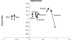
We applied the object splitting method to the Fats' and oils' data of Table 1. We used only four interval features. The contribution ratios of the first two principal components {"image_source":{"path":"images/372da338742b134f74ec4566896d2f80ea7ac7e82b60c6a419f15a3905f3cd62.jpg"},"content":"","chart_caption":[{"type":"text","content":"Fig. 4: The result of the SO-PCA for Fats' and oils' data (Pearson)."}],"chart_footnote":[]}
are 67.38% and 21.47% by the Pearson coefficient, and are 64.60% and 27.85% by the Spearman coefficient. Figs. 4 and 5 show the results of the SO-PCA based on the Pearson and the Spearman correlation matrices. These figures show the arrow line representation of eight objects in the factor planes. An arrow line connects from the minimum sub object to the maximum sub-object. The rectangle shown by dotted lines in Fig. 4 indicates the Cartesian join for Linseed oil that is the largest object. In Figs 4 and 5, the second principal component plays the size factor. On the other hand, in the first principal component, Specific gravity and Iodine value take positive weights, while Freezing point and Saponification value took negative weights. The mutual positions of the given eight symbolic objects are almost similar by the Pearson and the Spearman coefficients. However, we can see some differences in the lengths and the directions of some arrow lines by the Pearson and the Spearman coefficients. In this example, we should note that the arrow line representation supports a better {"image_source":{"path":"images/a7bfbb80f53d66f2ca426304073a1919bf416312e3411216d16c3b5e922d97d4.jpg"},"content":"","chart_caption":[{"type":"text","content":"Fig. 5: The result of the SO-PCA for Fats' and oils' data (Spearman)."}],"chart_footnote":[]}
understanding for the descriptions of symbolic objects in the factor planes compared to the rectangular representation.
Chouakria et al. [6] presented a comparative study of the vertices method (V-PCA) and the centers method (C-PCA). The V-PCA is implemented on the numerical data table of the size , while the C-PCA is implemented on the size . Therefore, the C-PCA is stronger than the V-PCA in the computational complexity, when the number of descriptive features is large. The contribution ratios of the first two principal components for the fats' and oils' data of Table 1 are 68.29% and 20.23% by the V-PCA, and 75.23% and 15.09% by the C-PCA, respectively. The rectangular representations of objects for these two methods are similar, although their contribution ratios are different. Moreover, their results are also close to the arrow line representations in Figs 4 and 5.
Lauro et al. [8] presented a comparative study of the V-PCA, the method called spaghetti PCA, and the method based on interval algebra and optimization theory. For the Fats' and oils' data of Table 1, their results of rectangular representations in the first factor planes are mutually similar. Among them, the spaghetti PCA is especially close to the result in Figs 4 and 5. The spaghetti PCA uses the main diagonals of the hyper-rectangles to represent multidimensional interval data. The contribution ratios of the first two principal components are and . In the representation of interval objects in the first factor plane, the lengths and the directions of the main diagonals of the rectangular regions are very similar to those of the arrow lines in Figs 4 and 5. The spaghetti PCA is a very different method from the object splitting method. However, we should point out the fact that the main diagonal of an object may be described by two end points: the minimum vertex and the maximum vertex.
In this section, we presented the object splitting method of PCA for interval objects. This method transforms the given interval-valued data table into a standard numerical data table, then executes the PCA on the transformed data table. We should note that
The object splitting method is simple and works as well as other methods for interval objects. Especially, this method is easily applicable to large data tables.
The arrow line representation of objects in the factor planes is useful to provide insights about the mutual relationships of the given interval objects.
In the next section, we present the quantile method, which is an extension of the object splitting method and can manipulate not only interval-valued features but also other type features including histogram features and nominal multi-valued features.
III. COMMON REPRESENTATION BY QUANTILES
In the aggregation process of large data sets, the use of histograms is very natural and common to describe the reduced data sets. Billard and Diday summarize empirical distribution functions and descriptive statistics for various feature types. Based on knowledge of distribution functions, the quantile method provides a common framework to represent symbolic data described by features of different types. The basic idea is to express the observed feature values by some predefined quantiles of the underlying distribution. In the interval feature case, a distribution is assumed within each interval, e.g., uniform distribution (Bertrand and Goupil ). For a histogram feature, quantiles of any histogram may be obtained simply by interpolation, assuming the uniformity in each bin of the histogram . Although the numbers of bins of the given histograms are mutually different in general, we can obtain the same number of quantiles for each histogram. For nominal multi-valued features, quantiles are determined from ranking defined on the categorical values based on their frequencies. Therefore, when we choose quartiles, for example, we can represent each feature value for different feature types in the same form of a 5-tuple (min,
). This common representation then allows for a unified approach to S-PCA. In the following subsections, we describe detail procedures to have quantile values for various feature types.
3.1. Quantiles for Interval-valued Feature
Let a feature be an interval-valued feature and let each object be represented by an interval:
We assume that each interval has a uniform distribution . Then, in the case of m quantiles, the resultant quantile values become
Therefore, each object for the feature is described by an -tuple:
{"image_source":{"path":"images/bbedbf94e7a7c5276eb8da233823618a32a57cc385e019fa01d024f639fc8174.jpg"},"content":"","chart_caption":[{"type":"text","content":"Fig. 6: A histogram-valued data."}],"chart_footnote":[]}
3.2. Quantiles for Histogram-valued Feature
Let a feature be a histogram feature and let an object be represented by a histogram in Fig. 6. Let the histogram be composed of bins, and let be the probability of the th bin, where it is assumed that . Then, under the assumption that bins (subintervals) have uniform distributions, we define the cumulative distribution function of the histogram [2,4] as:
Then, in the case of quantiles, we can find values including quantile values from the equations:
Therefore, the object is described by an -tuple
In general, we can describe each object under a histogram-valued feature by an -tuple:
It should be noted that the numbers of bins of the given histograms are mutually different in general. However, we can select an integer number m, and obtain -tuples as the common representation for all histograms.
3.3. Quantiles for Nominal (categorical) Multi-valued Feature
Let be a multi-valued feature which takes n possible categorical values . For each i, let be the relative frequency of categorical value in terms of N objects [2,4,15]. Then, we sort the relative frequency values. For simplicity, we assume that:
According to this order, we suppose rank values 1, 2,..., n for the categorical values , ,..., , respectively. We define the cumulative distribution function for each object based on the rank values.
Let be the number of possible categorical values taken by object under . Let be the frequency value associated with the category and given by
Therefore, we define a piecewise linear cumulative distribution function for each object based on uniform densities attached to rank values (see Example 4). Then we find values including quantile values for the selected integer number m. Therefore, we can obtain again the common -tuple representation:
EXAMPLE 4: The fifth feature (Major acids) of Table 1 is an example of nominal multi-valued feature. We suppose the quartile case, i.e. m = 4. For this purpose, we use basically the procedure given in the above. However, in order to prevent ties of rank values, we use the sums of frequency values attached to the category values of each object. Table 2 summarizes the results. From this table, the object Linseed, for example, has the minimum value four and the maximum value nine. Then, we assume uniform probability densities for the intervals associated with the ranking values:
where we should note that the interval is attached to the maximum rank value nine. The corresponding cumulative distribution function is a piecewise linear function characterized by:
By solving the equations , , and , we obtain the quartile values ,
| Object | Lu | A | C | Ln | M | S | P | L | O |
| Linseed | 0 | 0 | 0 | 0.2 | 0.2 | 0 | 0.2 | 0.2 | 0.2 |
| Perilla | 0 | 0 | 0 | 0.2 | 0 | 0.2 | 0.2 | 0.2 | 0.2 |
| Cotton | 0 | 0 | 0 | 0 | 0.2 | 0.2 | 0.2 | 0.2 | 0.2 |
| Sesame | 0 | 0.2 | 0 | 0 | 0 | 0.2 | 0.2 | 0.2 | 0.2 |
| Camellia | 0 | 0 | 0 | 0 | 0 | 0 | 0 | 0.5 | 0.5 |
| Olive | 0 | 0 | 0 | 0 | 0 | 0.25 | 0.25 | 0.25 | 0.25 |
| Beef | 0 | 0 | 0.2 | 0 | 0.2 | 0.2 | 0.2 | 0 | 0.2 |
| Hog | 0.167 | 0 | 0 | 0 | 0.167 | 0.167 | 0.167 | 0.167 | 0.167 |
| 0.167 | 0.2 | 0.2 | 0.4 | 0.767 | 1.217 | 1.417 | 1.717 | 1.917 | |
| Rank | 1 | 2 | 2 | 4 | 5 | 6 | 7 | 8 | 9 |
, and , respectively. Finally, we have the desired 5-tuple:
It should be noted that we are also able to treat other feature types such as discrete multi-valued features, binary features, etc., by assuming appropriate distribution functions.
IV. THE QUANTILE METHOD FOR S-PCA
Let be given objects. Let each object be described by d features. In general, d features are a mixture of interval features, histogram features, nominal multi-valued features and other types.
DEFINITION 9: Quantile sub-objects.
Let each object be described with the given features by -tuples:
Then, we define the quantile sub-object as:
PROPOSITION 7: For each object , the min imum sub-object , quantile sub-objects ( , , ), and the maximum sub-object organize a monotone structure in the space .
Proof: From the definition of sub-objects, we can obtain the following nesting relations of the Cartesian join regions:
Thus, Definition 7 leads the conclusion.
PROPOSITION 8: Property of correlation matrix S by the quantile method
Let a series of objects , , is mono tone in the space and let the correlation matrix be obtained by applying the Kendall or Spearman's rank correlation coefficients to the sub-objects of Definition 9. Then, the absolute value of each off-diagonal element of is large.
Proof: From Proposition 7, sub-objects for each of N objects organize always a monotone structure in any subspace of . Therefore, if the given series of objects is monotone, their nesting property restrict the order of sub-objects to be similar in any subspace of . This leads to the conclusion.
Now, the quantile method for general S-PCA is summarized as follows.
PROCEDURE 2: The quantile method for S-PCA Let the set of N objects be described by d features, which are a mixture of interval features, histogram features, nominal multi-valued features, and other types. Then, we execute the quantile method by the following steps.
We select an integer value ( ).
For each feature , we find the common representation of N objects by the -tuples:
For each object , we find -dimensional sub-objects: the minimum sub-object , quantile sub-objects, , ,..., , and the maximum sub-object . Then we split each object into sub-objects. As the result, we have an numerical data table. 4. We calculate the correlation matrix for the data table obtained in 3) based on the selected correlation coefficient, where we can use the Kendall or Spearman's rank correlation coefficient, or the Pearson correlation coefficient.
We find the principal components based on the correlation matrix in 4).
In the factor planes, we can reproduce each object , as a series of m arrow lines:
As a different representation, we can use also a series of m rectangles.
In this procedure, if we select as m = 1, the quantile method is reduced to the original "object splitting method".
V. EXAMPLES OF THE QUANTILE METHOD FOR S-PCA
EXAMPLE 5: Fats' and oils' data
We illustrate the quartile case, i.e. m = 4. In this case, the common representation of each object under a feature is 5-tuple, i.e. (min, , , , max). For the fifth feature Major acids, we used the quantification in Example 4. For the data in Table 1, we obtain the necessary 5-tuples for each of the eight objects with respect to five features. Then, we split each object into five sub-objects, i.e. the minimum sub-object, three quantile sub-objects, and the maximum sub-object. Therefore, we have 40 sub-objects for the given eight objects. Table 3 shows a part of our data, where five sub-objects are presented only for Linseed and Perilla. Table 4 shows the correlation matrices by the Pearson and Spearman coefficients. The elements of the upper triangular matrix show the Pearson correlation coefficients and those of the lower triangular matrix show the Spearman correlation coefficients. For the Spearman coefficient, Specific gravity and Iodine values show the highest correlation, while, for the Pearson coefficient, Specific gravity and Freezing point values show the negatively highest coefficient. We can find another difference between the Spearman and the Pearson coefficients for the correlation between Saponification and Major acids values.
Figs. 7 and 8 show the results of the S-PCA based on the Pearson and Spearman correlation matrices. The contribution ratios of the first two principal components are 56.28% and 26.68% by the Pearson coefficient, and are 53.71% and 34.54% by the Spearman coefficient. Each object is described by a series of four arrow lines. In this example, the second principal component plays the role of the size factor, and Major acids and Saponification value take especially large positive weights. On the other hand, in the first principal component, Specific gravity and Iodine values take large positive weights, while Freezing point and Saponification values took large negative values.
| Linseed | |||||
| 1 | 0.93000 | -27 | 170 | 118 | 4 |
| 2 | 0.93125 | -24.75 | 178.5 | 137.5 | 5.25 |
| 3 | 0.93250 | -22.5 | 187 | 157 | 7.5 |
| 4 | 0.93375 | -20.25 | 195.5 | 176.5 | 8.75 |
| 5 | 0.93500 | -18 | 204 | 196 | 10 |
| Perilla | |||||
| 1 | 0.93000 | -5 | 192 | 188 | 4 |
| 2 | 0.93175 | -4.75 | 196 | 190.25 | 6.25 |
| 3 | 0.93350 | -4.5 | 200 | 192.5 | 7.5 |
| 4 | 0.93525 | -4.25 | 204 | 194.75 | 8.75 |
| 5 | 0.93700 | -4 | 208 | 197 | 10 |
| S | Spec. | Freez. | Iodine | Sapon. | M. acids |
| Spec. | 1.0000 | -0.8923 | 0.7682 | -0.3187 | 0.2432 |
| Freez. | -0.6309 | 1.0000 | -0.6368 | 0.4968 | -0.1138 |
| Iodine | 0.9582 | -0.6142 | 1.0000 | -0.3834 | 0.1107 |
| Saponi. | -0.2044 | 0.6437 | -0.1980 | 1.0000 | 0.3634 |
| M. acids | 0.2558 | 0.0398 | 0.1805 | 0.6428 | 1.0000 |
By the addition of Major acids, the lengths of objects became larger than those in Figs 4 and 5. The position of Camellia moved slightly towards the upper side. The mutual positions of eight objects are almost the same in Figs 7 and 8. However, some differences exist in the sizes and the directions of arrow lines.
EXAMPLE 6: Histogram data (Hardwood data)
The histogram data used here are selected from the US Geological Survey (Climate-Vegetation Atlas of North America [16]). The number of objects is 16 and the number of features is eight. Table 5 shows histogram values for 16 hardwoods under the feature: Annual temperature (ANNT). In this table, N is the number of preselected regions in which the hardwood exists. For example, Acer East is observed in 6869 regions. The ANNT of these 6869 regions is in the range from -2.3 to 23.8°C. In other words, 100% of 6869 Acer East samples exist in the range from -2.3 to 23.8°C, while 50% of 6869 samples exist in the range between -2.3 and 9.2°C, and so on. We selected the following eight features to describe objects (hardwoods). The data formats for other features are the same with Table 5, viz.,
: Annual temperature (ANNT) (°C);
: January temperature (JANT) (°C);
: July temperature (JULT) (°C);
: Annual precipitation (ANNP) (mm);
: January precipitation (JANP) (mm);
: July precipitation (JULP) (mm);
: Growing degree days on C base 1000 (GDC5); and
: Moisture index (MITM).
In this example, deciles and quartiles describe each object, where the preselected number m is 6, and the 7-tuple is used as a common representation for the given Ichino: The Quantile Method for Symbolic PCA 195 {"image_source":{"path":"images/49d78214bf4b4c8cbcf05fa8112eb147426cb712c5ec324b8ce09702b4d7c87d.jpg"},"content":"","chart_caption":[{"type":"text","content":"Fig. 7: The result of the S-PCA for Fats' and oils' data (Pearson)."}],"chart_footnote":[]}
16 hardwoods. According to the Procedure 2 for S-PCA in Section 4, we transform the given (16 objects) × (8 features) symbolic data table to a sub-objects) × (8 features) standard numerical data table. Table 6 shows a part of the transformed data table.
Table 7 shows the correlation matrices, where the upper triangular matrix shows the elements of the Pear son correlation matrix, and the lower triangular matrix shows the elements of the Spearman's rank correlation matrix. The Pearson and the Spearman correlation matrices are similar in many elements. However, some differences should be pointed out. Features (ANNT), (JANT), (JULT), and (GDC5) are highly correlated mutually for the Spearman coefficient. Feature (ANNP) is strongly correlated with features (JANP) and (MITH) for the Spearman coefficient, while (ANNP) is largely cor related with features (JANP) and (JULP) for the Pearson coefficient. We see also a difference between the Pearson and Spearman correlation coefficients concerning feature (GDC5).
The contribution ratios of the first two principal components are 77.01% and 11.64% for the Pearson correlation matrix, and are 87.41% and 8.38% for the Spear man correlation matrix. Figs 9 and 10 show the arrow {"image_source":{"path":"images/21d0dff3a86a62e0da847301fd961b13041e905818397a6037f6be03b3b46cd4.jpg"},"content":"","chart_caption":[{"type":"text","content":"Fig. 8: The result of the S-PCA for Fats' and oils' data (Spearman)."}],"chart_footnote":[]}
| Taxon name | Annual temperature (°C) | |||||||
| N | 0% | 10% | 25% | 50% | 75% | 90% | 100% | |
| Acer East | 6 865 | -2.3 | 0.6 | 3.8 | 9.2 | 14.4 | 17.9 | 23.8 |
| Acer West | 1 954 | -3.9 | 0.2 | 1.9 | 4.2 | 7.5 | 10.3 | 20.6 |
| Alnus East | 10 144 | -10.2 | -4.4 | -2.3 | 0.6 | 6.1 | 15.0 | 20.9 |
| Alnus West | 4 761 | -12.2 | -4.6 | -3.0 | 0.3 | 3.2 | 7.6 | 18.7 |
| Betula | 16 815 | -13.4 | -8.4 | -5.1 | -1.0 | 3.9 | 12.6 | 20.3 |
| Carya | 4 638 | 3.6 | 7.5 | 10.0 | 13.6 | 17.2 | 19.4 | 23.5 |
| Castanea | 2 216 | 4.4 | 8.6 | 11.3 | 14.9 | 17.5 | 19.2 | 21.5 |
| Fraxinus East | 8 565 | -2.3 | 1.4 | 4.3 | 8.6 | 14.1 | 17.9 | 23.2 |
| Fraxinus West | 1 095 | 2.6 | 9.4 | 11.5 | 17.2 | 21.2 | 22.7 | 24.4 |
| Juglans East | 4 138 | 1.3 | 6.9 | 9.1 | 12.4 | 15.5 | 17.6 | 21.4 |
| Juglans West | 526 | 7.3 | 12.6 | 14.1 | 16.3 | 19.4 | 22.7 | 26.6 |
| Ostrya/Carpinus | 5 348 | 1.2 | 4.4 | 7.0 | 11.4 | 16.0 | 19.2 | 28.0 |
| Quercus East | 7 360 | -1.5 | 3.4 | 6.3 | 11.2 | 16.4 | 19.1 | 24.2 |
| Quercus west | 1 942 | -1.5 | 6.0 | 9.5 | 14.6 | 17.9 | 19.9 | 27.2 |
| Tilia | 3 792 | 1.1 | 3.8 | 5.8 | 8.8 | 12.0 | 14.4 | 19.9 |
| Ulmus | 8 028 | -2.3 | 1.7 | 4.9 | 9.7 | 15.3 | 18.6 | 23.8 |
| Taxon name | ||||||||
| Acer East | ||||||||
| 1 | -2.3 | -24.6 | 11.5 | 415 | 10 | 56 | 0.5 | 0.62 |
| 2 | .6 0 | -18.3 | 16.6 | 720 | 23 | 77 | 1.2 | 0.89 |
| 3 | .8 3 | -12.3 | 18.2 | 835 | 40 | 89 | 1.5 | 0.94 |
| 4 | .2 9 | -5.1 | 22.2 | 1010 | 69 | 100 | 2.5 | 0.97 |
| 5 | .4 14 | 2.3 | 25.8 | 1200 | 96 | 113 | 3.6 | 0.99 |
| 6 | .9 17 | 7.9 | 27.3 | 1355 | 127 | 135 | 4.8 | 0.99 |
| 7 | .8 23 | 18.9 | 28.8 | 1630 | 166 | 222 | 6.8 | 1.00 |
| Acer West | ||||||||
| 1 | -3.9 | -23.8 | 7.1 | 105 | 5 | 0 | 0.1 | 0.14 |
| 2 | .2 0 | -11.8 | 11.3 | 380 | 28 | 8 | 0.5 | 0.49 |
| 3 | .9 1 | -10.1 | 12.8 | 505 | 54 | 23 | 0.7 | 0.61 |
| 4 | .2 4 | -6.9 | 14.9 | 750 | 92 | 38 | 1.1 | 0.75 |
| 5 | .5 7 | -1.3 | 17.6 | 1175 | 176 | 52 | 1.6 | 0.91 |
| 6 | .3 10 | 3.3 | 19.9 | 1860 | 267 | 71 | 2.2 | 0.98 |
| 7 | .6 20 | 11.0 | 29.2 | 4370 | 616 | 160 | 5.6 | 1.00 |
| Alnus East | ||||||||
| 1 | -10.2 | -30.9 | 7.1 | 220 | 9 | 28 | 0.1 | 0.22 |
| 2 | -4.4 | -26.5 | 13.2 | 380 | 19 | 58 | 0.6 | 0.53 |
| 3 | -2.3 | -22.7 | 14.8 | 475 | 23 | 74 | 0.8 | 0.69 |
| 4 | .6 0 | -18.1 | 16.5 | 770 | 46 | 91 | 1.1 | 0.93 |
| 5 | .1 6 | -8.0 | 19.8 | 1060 | 80 | 108 | 1.9 | 0.99 |
| 6 | .0 15 | 3.7 | 25.7 | 1235 | 106 | 126 | 3.7 | 0.99 |
| 7 | .9 20 | 14.1 | 29.1 | 1650 | 166 | 212 | 5.9 | 1.00 |
| Alnus West | ||||||||
| 1 | -12.2 | -30.5 | 7.1 | 170 | 4 | 0 | 0.1 | 0.22 |
| 2 | -4.6 | -25.7 | 11.5 | 335 | 18 | 21 | 0.5 | 0.49 |
| 3 | -3.0 | -21.6 | 12.8 | 410 | 23 | 41 | 0.7 | 0.59 |
| 4 | .3 0 | -15.1 | 14.4 | 510 | 37 | 57 | 0.9 | 0.72 |
| 5 | .2 3 | -7.6 | 15.6 | 790 | 93 | 74 | 1.1 | 0.87 |
| 6 | .6 7 | -0.8 | 17.5 | 1385 | 199 | 87 | 1.6 | 0.97 |
| 7 | .7 18 | 10.8 | 28.3 | 4685 | 667 | 452 | 4.8 | 1.00 |
| S | ANNT | JANT | JULT | ANNP | JANP | JULP | GDC5 | MITM |
| ANNT | 1.0000 | 0.9836 | 0.9666 | 0.6524 | 0.5633 | 0.7573 | 0.9584 | 0.6381 |
| JANT | 0.9851 | 1.0000 | 0.9190 | 0.6354 | 0.5635 | 0.7438 | 0.9424 | 0.5754 |
| JULT | 0.9706 | 0.9242 | 1.0000 | 0.6856 | 0.5888 | 0.7673 | 0.9329 | 0.7477 |
| ANNP | 0.8154 | 0.7746 | 0.8660 | 1.0000 | 0.9349 | 0.8237 | 0.6695 | 0.6154 |
| JANP | 0.7828 | 0.7689 | 0.8139 | 0.9548 | 1.0000 | 0.7062 | 0.5854 | 0.4704 |
| JULP | 0.8356 | 0.7834 | 0.8859 | 0.8999 | 0.8149 | 1.0000 | 0.8302 | 0.6360 |
| GDC5 | 0.9934 | 0.9650 | 0.9837 | 0.8211 | 0.7744 | 0.8635 | 1.0000 | 0.5792 |
| MITM | 0.7268 | 0.6678 | 0.8079 | 0.9569 | 0.8798 | 0.8899 | 0.7458 | 1.0000 |
{"image_source":{"path":"images/ca680f8cc6a1991f2c129c1aa2afe930a41a72e15888944e9b309a35a713c24e.jpg"},"content":"","chart_caption":[],"chart_footnote":[]} {"image_source":{"path":"images/5cf80f9d2cada17eaef8809722efb5d6008b7b40959fc0d49fd5c2a0dccb5169.jpg"},"content":"","chart_caption":[{"type":"text","content":"Fig. 9: The result of the S-PCA for hard woods (Pearson)."},{"type":"text","content":"Fig. 10: The result of the S-PCA for hard woods (Spearman)."}],"chart_footnote":[]}
line representations of sixteen hardwoods in the factor planes by the Pearson and Spearman correlation matrices, respectively. In the two factor planes, the first principal component plays the role of the size factor, and the given eight features take similar positive weights. In the second principal component, four features concerning precipita tion and moisture, i.e. ANNP, JANP, JULP, and MITH, take positive weights, while other features for temperature and growing degree, i.e. ANNT, JANT, JULT, and GDC5, took negative weights. For the Spearman correlation matrix, moisture (MITH) takes an especially large positive weight for the second principal component. However, for the Pear son correlation matrix, the corresponding weight is very small.
In Fig. 9, many series of arrow lines tend to be slightly right down. Almost all kinds of hardwood in the eastern area of the US organize a large stream of arrow lines. This tendency of the main stream depends on temperature and precipitation. On the other hand, largely fluctuating and mutually separate streams are mainly composed of the hardwoods in the western area. For example, Acer West, Alnus West, Betula, and Fraxinus West most drastically change toward the upper right with the last decile. This change is heavily dependent on precipitation and moisture. In Fig. 10, the main stream of arrow lines has two branches. Each branch initially grows toward the upper right, and then changes direction toward right down. This property is not clear in Fig. 9. Generally, mutual arrow lines are clearly represented in Fig.
- Therefore, in this example, the Spearman correlation matrix may be better than the Pearson correlation matrix. Since the quantile method is based on the monotonic property of the given set of objects, the use of the Spearman correlation matrix may be natural.
VI. CONCLUDING REMARKS
We presented the quantile method for the S-PCA. The quantile method can treat not only histogram-valued data, but also nominal and ordinal multi-valued type data, and is simply based on the property of monotone structure of the given objects. By selecting a common integer number m, the quantile method transforms a given complex symbolic data table to a simple numerical data table. An important aspect is that we can select the integer m as a sufficiently small number compared to the number N of objects, and we can apply the traditional PCA simply to the data table. We presented several experimental results in order to show the effectiveness of the quantile method. An arrow line representation of objects in the factor plane may be a useful tool to analyze complex symbolic data tables.
ACKNOWLEDGMENTS
This research was partly supported by Japan Society of the Promotion of Science (Grant-in Aid for Scientific Research (C) 19500130). The author wishes to thank referees and editors for suggestions leading improvements in this article. The author also acknowledges to Professor Paula Brito for her collaborations.
Conflict of Interest
The authors declare no conflict of interest.
Ethical Approval
Not applicable
Data Availability
The datasets used in this study are openly available at [repository link] and the source code is available on GitHub at [GitHub link].
Funding
This work did not receive any external funding.
References
Cite this article
Related Research


Special Issue
Launch a focused special issue to highlight research, emerging trends, and expert insights in your academic field.