What’s Inside of a Black-Hole in AdS Space

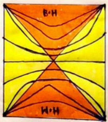
# I. INTRODUCTION In this paper I wanna talk about I decided not to give a broad introduction on "Complexity and Black-holes", just focus on some particular problem, which have been concern to me sometimes a problem on what the black holes do, how do they behave (The interior, when I speak about black hole, I usually mean the Interior of the black hole.) at exponential amount of time. Exponential time means exponential amount of entropy! So there is a very good reason to believe that something different, something perhaps you may call a break-down of "Standard Classical General Relativity", happens inside of a blackhole (at exponential time)! So how do we describe it??? That's I think not known, not well known (I mean, we don't know well) what happens and, I like to discuss the basic idea, whenever I wrote any paper! I'm not a rigorous mathematician! But, I have some usual sense, between what I write and what I think! In this particular problem, I don't know how long I write or talk about??? Because, it's a big and interesting problem, about the relationship between quantum mechanics and gravity! So, here we have a penrose diagram for black hole (See fig: a)! Lower part of this figure called "Whitehole", and the upper part is called the "Blackhole" region! And I fill-up the diagram with space-like surfaces! And those space-like surfaces are anchored with the AdS-boundary! This figure has (see fig: a) two sided static spatial boundaries, that means it can be described by the two copies of Conformal Field Theory! The region between to the left-horizon and right-horizon, you can think of as a Wormhole, connecting two sides! An worm-hole just a growing volume! You can see it from the "figure: a!" The volume of the worm-hole at the middle is "Zero"! Then it growing and growing, in fact if you looked at the corners (what's going on), it growing for very long time to enormously large, classically it just grows forever or tends to infinity! And on the white-hole side, the opposite thing happens, from a very large volume it shrink-down! And the puzzle that i confused for five and a half year; what the meaning of this entire process??? Because, if you stand outside from the black hole and observe it, the black-hole completely stationery! And it completely clear that it doesn't have to do, growth and shrink of entropy during a "Boltzmann Fluctuation" or anything like that (it doesn't have to do with entropy!). So it's have to do something else! I think we now, have a large amount of evidence of some form of complexity is responsible for this kind of process! So, what do we know from this space like surfaces??? The spatial volume of them grows linearly with time and the coefficient $A_h$ confirms, that linear growth ( $A_h$ : is the area of the horizon)! $$ \mathrm{V} = \mathrm{A}_{\mathrm{h}} \cdot \mathrm{t} $$ That the one thing we know! Other thing that i strongly suspect is that, the complexity of a quantum state (The quantum state of the boundary theory) also grows linearly for some period of time: $$ \mathrm{C} = \mathrm{S} \cdot \mathrm{T} \cdot \mathrm{t} $$ And the coefficient which confirms that linear growth is proportional to the entropy (S) of blackhole $\times$ the temperature (T)! That is actually a guess, not a rigorous statement! But it's seems to work very well. So if we put this two-formula together and use a little bit of information about the geometry; we find the complexity given by the volume of the worm-hole (V) divided by Newton Constant (G) times AdS-radius! $$ C = V / [ G \cdot l_{ads} ] $$ So, complexity proportional to the volume! Now what did we mean by complexity??? Normally the usual way, to think about complexity: How many gates or how many elementary operation does it take to produce a certain quantum state (From a reference state which is in some sense very simple)??? So the evolution of state, is also proportional to the number of gates or operations! In other words, we can Say complexity is the number of circuit elements or how hard it is to bring the state back into some simple state! Equivalently In terms of worm hole, how complicated, how difficult it is, to restore, to shrink the worm-hole back to something very small! It's doesn't matter which way you think about "The Complexity"! It's like taking some worm-hole very big and shrunken-down for some purpose to smallest possible "worm-hole", then the complexity measure in terms of "How hard to do that"!!! 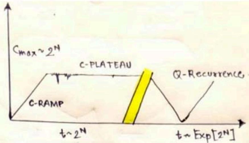So, now let's focus on the Complexity-curve! It's a conjecture curve! Which we certainly don't know for sure that it's exactly right! But i will assume that; it close to being right! The complexity as a function of time. First, we start with the "Zero Complexity State", i mean the "TFD"/"Thermal Field Double" state, then it's (complexity) start to increase linearly! I called it linear increase complexity ramp or "C-ramp". And, according to the formula it takes place for an exponential time (as expected)! I will say; $2^{\mathrm{n}}$ (2 the power n, n: is the number of q-bits that describe the system)! But complexity does not increase as we expected, since the complexity bounded above $2^{\mathrm{n}}$ -limit (see the fig: b)! So the complexity is now flattened-out, i call it: complexity plateau or "C-plateau" (see the fig: b)! That complexity plateau stays for enormous amount of time! It's kind of equilibrium but it's kind a super equilibrium, way way beyond the thermal equilibrium! And it lasts for very very long time, double exponential in the number of q-bits [t~exp(2n)] But on that time-scale, "recurrence" can happen! Yes it does happen! Recurrence are more accidental return of the system into original state! Of course it's much more likely that you have a partial recurrence ; but I'm interested now in the full recurrence! The full recurrence is go all the way back, and as i said it's incredibly a rare phenomena! But one of the reason, I'm interested in; especially on recurrence is because it's my claim that a quantum recurrence is describe exactly by the penrose diagram that you see before! The white-hole, the black-hole that is exactly the quantum recurrence! It's last a amount of time: $2^{\mathrm{n}}$ (simple exponential); but it take's place in a "C", long long "C" of time (Grand Range Of Time) that this quantum recurrence is happen double exponential time $\exp(2^n)$ : rarely! Now, what do i think??? I think that it's only during this quantum recurrence that the classical description of worm-hole actually makes sense! So i would, kept that view: "The Full Kruskal Diagram" (including black-hole, white-hole) is really a picture of quantum recurrence! And the life of the black-hole is mainly spent (I'm talking about eternal black-hole, not the evaporating one, means eternal black-hole in AdS-space) in this Complexity-equilibrium, or this "Complexity/C-plateau"! Where noting much happen! It's just sit there, and doing very interesting phenomena that i can be describe classically and the view i gonna proposed in a moment! So the question is: "what happened to the worm-hole at the transition point, between the complexity ramp and complexity plateau??? So what is happening, i mean what is happening according to the "bulk worm-hole" point of view? What happens to worm-hole at exponential amount of time??? And you can also think it in terms of what going on during the long period of equilibrium on the "plateau"? How do we describe it? I can give you some possible number of answers; firstly "Just Keep Growing"! The just keep growing theory says: "Nothing happens there, it just keep growing!!!" The whole idea using complexity as a marker for worm-hole size just breaks-down! And the worm hole doesn't care all about complexity, just keep growing. I think it's wrong point of view, but though it's just one possible answer! 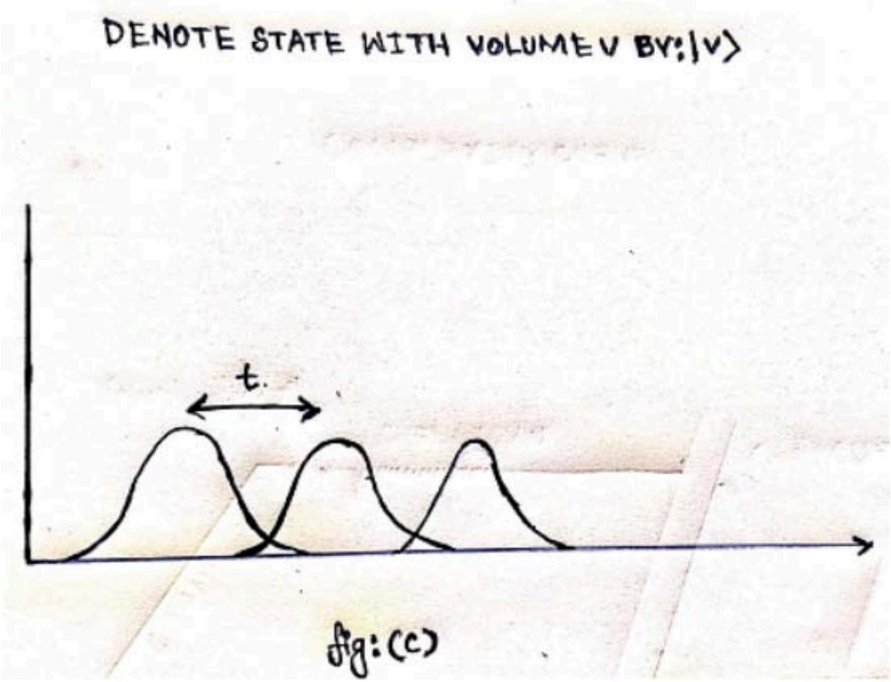Anyway, it can be called the "pseudo-complexity". But the other possible answer is; it's stop growing, that intact you can't extend complexity equal volume or C~V, for an exponential amount of time. So if that's true, then is it transition sudden or gradual. In either case, what is the geometry of the interior on the "C-plateau"???? Is there any geometry or it's just a terrible quantum-mechanical mess of complexity??? Actually the geometry doesn't even make any sense! That's are the questions that i like to answer!!! Or, may be just speak about some partial answers! The partial answers are less like to be report; but i can do as much as i can! Okay, let's denote a state of a worm-hole with volume: V by a ket state: |V\rangle I want to think the evolution of the state as V-increases (Volume increase)! I wanna think it as a sequence of state in which the volume changes by an amount which is perceptible and measurable! Which means that, the wave function is the function of volume, goes through a sequence almost orthogonal states! The time it takes for a state go itself to something, which is almost orthogonal i called the "Haar-bounded" time. As i learn it from "Haranov"! And we can think of the evolution as a sequence of states which are classically distinguishable from each other, or at least distinguishable from each other. And that sense they define a clock! The volume defines kind of clock variables! But eventually you, run out of states! Why that??? Because the hilbert space of the black hole has finite dimensionality! The dimensionality is roughly $\sim 2^{n}$ of the black hole, means $2^{n}$ [n: the number of q-bits]! And eventually you run out of orthogonal states! If the theory was integrable, you might expect what happens??? What happens with an ordinary-clock who's states are periodic??? And if you ho some certain amount of time, you get to just before mid-night and just after mid-night [the clock jumps back one clock on exponential time scale, see the figure: c!] That's you would expect if the energy levels were exactly equally spaced! Then the system must be integrable! But that does not how the chaotic system behave! Chaotic system [ just tell you, the way chaotic system are expect to behave, is: "once you reach the exponential amount of time (so you run out of states), the new state of the system beyond that becomes a linear superposition of all the previous states!] On other words, try to make a Wormhole longer than the exponential, you get defeated, and instead, you make a linear super-position of states, of all of the worm-hole lengths with more or less equal probability! Now, that is something i have not seen any paper on worm-hole complexity, i just learnt it by doing thought experiment by myself, but it's may be well known to many people, i think!!! $$ | \Psi \rangle = \sum f (V) \cdot | V \rangle $$ $$ \mathrm{f}^{*}(\mathrm{V}) \cdot \mathrm{f}(\mathrm{V}) \approx \mathrm{e}^{-\mathrm{s}} $$ Here, N runs from 1 to $2^{n}$ . Okay! now this is firstly represent the volume of worm-hole; and after a certain amount of time, we see what happens: become a superposition of many many different classical state of the worm-hole! Is that mean, there is a sudden breakdown of classical general relativity??? The classical states don't mean anything! There is no geometry just the super-position of geometry??? I don't think so!!! I think this is somewhat misleading! I will tell you why, as i go long! But i come back that later (just keep it in mind)! I think, the right thing to understand this "Complexity Geometry"! By complexity geometry, i mean the thing L. Susskind and his collaborators invented! I don't go through the details on it, i just use it in a way to describe "black hole". But if you want to know more about it please visit "The 2nd Law of Complexity" by L.Susskind. And what i really gonna do is a "toy-model" of it; thats come from Brown-Susskind, and A.Hao "toy-model"! The "toy-model" is useful highly rigorous, but easy to understand! Okay, before we talk about that, lets talk about "complexity in unitary matrices". Unitary matrices have two rows! One row represent the unitary operators! Unitary Matrices $=$ Unitary Operators $$ U_{ij} = | i \rangle \langle j | $$ "U" of course the element of $SU(2^n)[U \in SU(2^n)]!$ The unitary operator acts on the space of $n \sim Q$ bits ($n \sim S$). So, one thing we do is to make unitary operators! The other thing we do with the same unitary matrices, that they represent the maximum entangled states! I think i don't need to explain that. $U_{ij}$ , where i, j may be some basis, sometimes called computational basis! So, what is Complexity geometry??? Complexity geometry is simply a geometry on the space of unitaries: $\mathrm{SU}(2^n)$ . But there is many geometry such on space; and there is very standard one "Bi-invariant Geometry" [I mean Left-Right invariant geometry]; and that's not the one which represent the complexity. The geometry that represent the complexity; is a geometry which you can start with a usual Matrix [Bi-invariant one] and then stretched those directions; which corresponds to difficult direction to move in. The difficult direction of move-in, once which is generated by Hamiltonians in which each-term involves simultaneously many many Q-bits. On other words, non-k-local Hamiltonian! You stretched the directions, make them very costly in length, the directions which you think of hard-directions, and leave small other directions. That pretty much, that i can speak about: "The notion of a penalty factor"! Penalty factor is a stretching factor, where you stretched out the geometry in a great deal of length; And the directions you want to think of as highly complex. So, what we know about such "Complex Geometry"?... First of all it's homogeneous! Homogeneous means same as every where! And i didn't inherent the homogeneity from the group structure $\mathrm{SU}(2^n)$ . But it also right invariant [as supposed to "Bi-invariant", and if you don't know what it mean just ignore it!] It has a diameter (diameter means, the largest distance between points) of order $2^n$ . Now, you may be surprised by $2^n$ . And that's represents simply the maximum complexity! The largest distance between points; or the distance to the identity operator represent the complexity of unitary! The volume of Complexity geometry is much much bigger, the volume is about $\sim \exp(2^n)$ . So the diameter is the logarithm of volume "D = log(V)". Now that is a characteristics of negatively curved spaces, as you move out the volume grows exponentially with the diameter. The another feature of complexity geometry is they negatively curved, or has some particular sectional curvature. Sectional curvature is the curvature of 2d surfaces! All the geometry/most of the geometry are negatively curved. That means; when you start out with geodesics, they deviate from each other rapidly or exponentially, and that is a sign of quantum chaos. Means, complexity geometry is negatively curved. And finally "the cut locus". 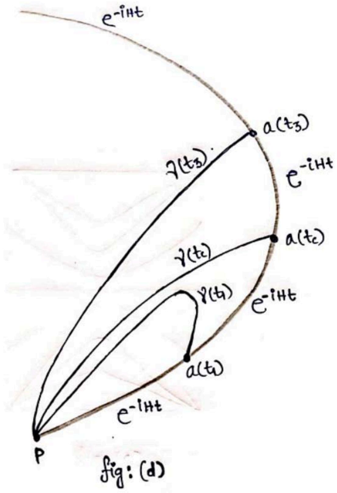This is a guess, and also a conjecture about what a complexity geometry should do. The cut locus, is far away from the identity, as it could possibly be, which means the diameter "D" of geometry. I haven't told you what cut locus is, so now I'm going to tell you. If you know the graph theory, you might begin to suspect that this sequence of five things here is very similar to the definition of a "expanded graph"?! Diameter-Volume connection, negatively curved space and so forth, it's a good analogy but if you don't know what a expanded graph is, i not gonna use it. So now, what is the meaning of a cut-locus??? Let me tell you, what cut locus is! Because i thing it's play a central role of my story! The cut-locus of a point is the collection of all cut-points related to that point. So what is a cut-point? Take a geodesic straight at point "p" (the cut-locus of point "p" or the cut points associated with "p")! Take a geodesic in the geometry, in the complexity geometry or any other geometry, and take a geodesic through it, or starting at it! Now lets label that geodesic $\mathsf{a}(\mathsf{t})$ . a: just represent a point, and t is just the parameter along the curve. It could be the time, but let's assume it's a some kind of parameter. Could be the length of the curve itself [The length of time you may consider]. You can expect that, for some sufficiently short time that geodesic that i have drawn (see the figure: d) is the shortest geodesic connecting p with $\mathsf{a}(\mathsf{t})$ ! You can always be sure, for some length of time any given geodesic is the shortest geodesic that Connects the point a. But at some point typically that a labeled $\mathsf{t}_{\epsilon}$ (c: for cut), the another geodesic of equal length $\gamma (\mathsf{t}_{\epsilon})$ will emerged and it's cross $\mathsf{a}(\mathsf{t})$ ! Let's imagine, there is some Short's of obstacles, it may be the topological obstacles or a big hill in the geometry that you have go around (see fig: d) There may other geodesic in addition the big geodesic (which goes around the hill). But typically for short times, that 2nd geodesic that point "p" with $\mathsf{a}(\mathsf{t})$ could be longer than the primary geodesic I'm started with! But as you let "t" increase, typically you would come to a point where some other geodesic $\gamma (\mathsf{t}_{\epsilon})$ will have the same length as the primary geodesic, beyond that $\gamma (\mathsf{t})$ is shorter than the primary geodesic! In other words; you reach a point, in which the shortest geodesic connecting "p" with "a", is a member of family $\gamma (\mathsf{t})$ : that point is called "cut-point". And the "cut-locus" is the collection of all cut-points that you get by sending any number of geodesic from the point "p". The cut-point represent a transition, in the behavior of shortest geodesic. If the shortest geodesic represent the complexity; then the cut-locus or the cut-points are the points; in which the character of the shortest geodesics discontinuously changes; the length of the shortest. The length of the shortest geodesic doesn't discontinuously change, it's contentious but the first derivative of it's does! # II. DISCONTINUOUS FUNCTION # L[p, a(t)] IS CONTINUOUS AT CUT POINT BUT (dL/dt) IS NOT!!! And so, something starts to happen to the shortest geodesic at the cut locus. Why it's interesting??? Because, if the length of geodesic represent complexity, and if complexity something has to do, with the Interior of the black holes, then the cut locus is the place, where the sudden sharp phenomena or transition can potentially take place! Let's go further! I have drawn here (see fig: d), I don't know what I called??? May be 2nd order cut. 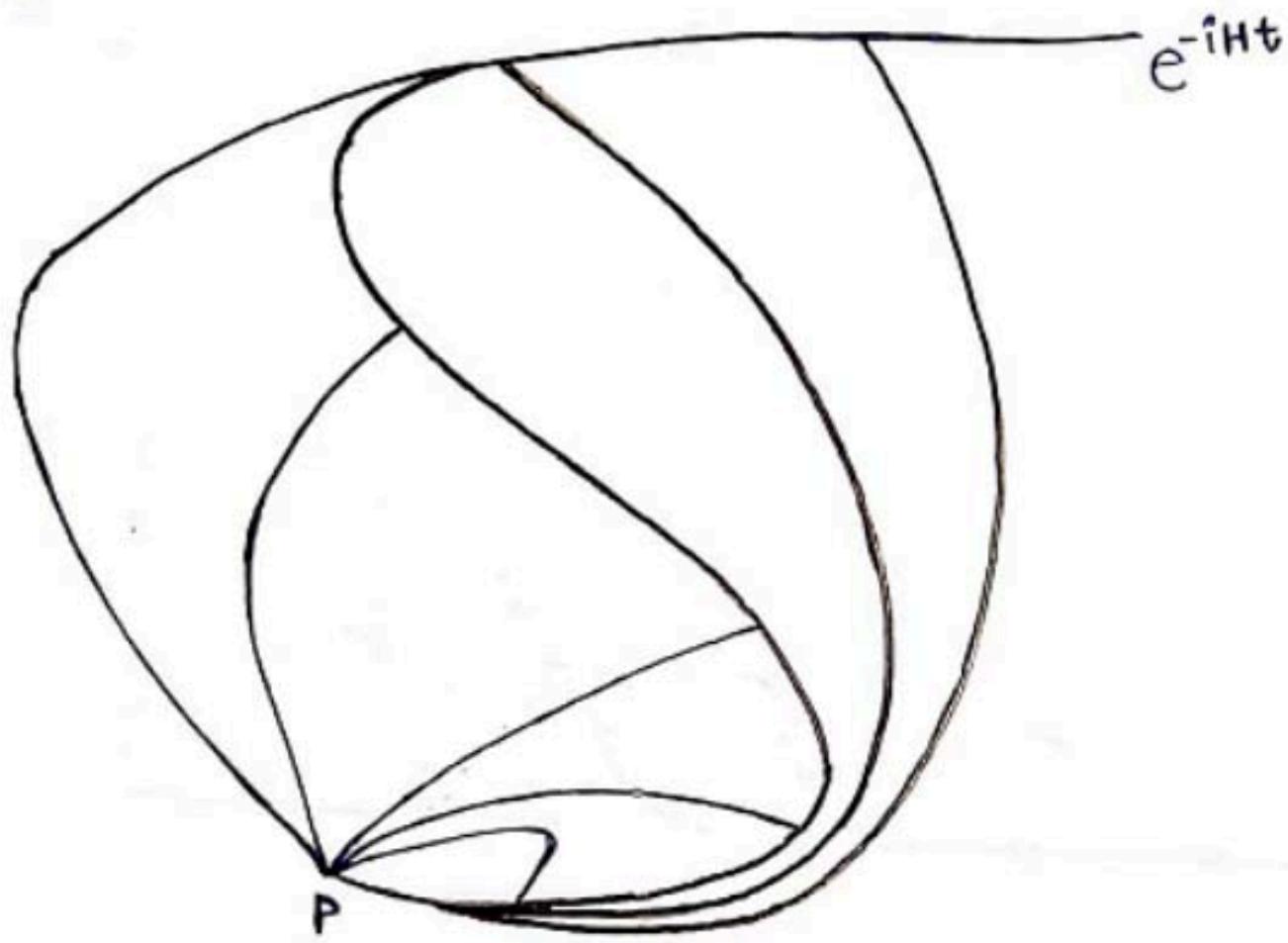Now again starting with "p" you go little ways, and you come to the cut-locus; with a "black-family" (incidentally notice that, the shortest geodesics after the cut-point not a single geodesics, anymore but a family of geodesics), and as you move along the main curve the sequence of "black-curves" are the shortest geodesics until you come to a 2nd point! At some 2nd point, the "geodesic" that through different obstacles, might suddenly emerged as shortest geodesic! And so for a typical geometry you find a whole sequence of cut points like this, and rather complicated answer of this question of cut-points like this (see fig: e), and rather complicated answer of geodesic this question how the energy of the shortest geodesics vary as you increase t/time. It doesn't even have to vary monotonically incidentally. The shortest geodesic can get shorter for a period of time [even though the main-curve get longer]! So, that's sequence of curves represent the transition in the behavior of shortest geodesics (see fig: e). Okay, now i wanna come to the "Toy model of complexity geometry"! Apply, this idea for "cut-locus", to a model of complexity geometry. The model is first proposed by Brown, Susskind, and Z.Hao! 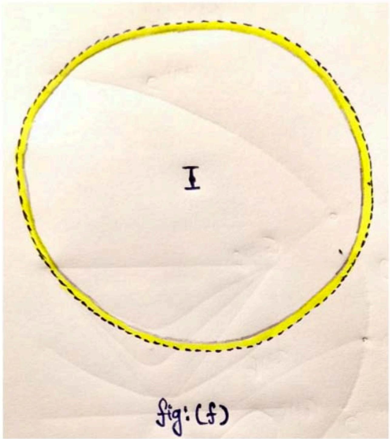It seems to rather good job, even though it's tremendously simplified, simplified down to 2d. So it's kind a good job, represents a lot of what you expect from complexity. Okay, so what is the model??? The model is "The Poincaré disc". 2d, uniformly-negative curved surface mapped on to a disc (which is 2d)! On this disc i also want to put an inscribed polygon. The side of the polygon is geodesic. They are geodesic on a negatively curved space! And on the top of everything else we gonna make an identification (see Made with Xodo PDF Reader and Editor fig: f)! Make identification by identify the sides randomly. Now you have to be a little bit of careful, there is one constraint, that you don't make conical singularities (it's a small constrain, you can satisfy it)! But up to that constraint you are allowed to make random identification. So how many sides there? The number of sides: $$ \begin{array}{l} \mathrm {S I D E S} = 4 \times [ \text {GENUS OF THE RIEMANN SURFACE} ] \\ = \text {Area of Total Riemann Surface}. \\ \approx \exp [ 2 ^ {n} ] \\ \end{array} $$ So the "Number of sides"~4 GENUS $\sim$ AREA; " $\rightarrow$ all three of are enormously large, the exponential of $2^{n}$ ! Now that's connected to the fact that the volume; of $\mathrm{SU}(2^{n})$ is exponentially large! And I want to represent that volume, of $\mathrm{SU}(2^{n})$ is exponentially large. 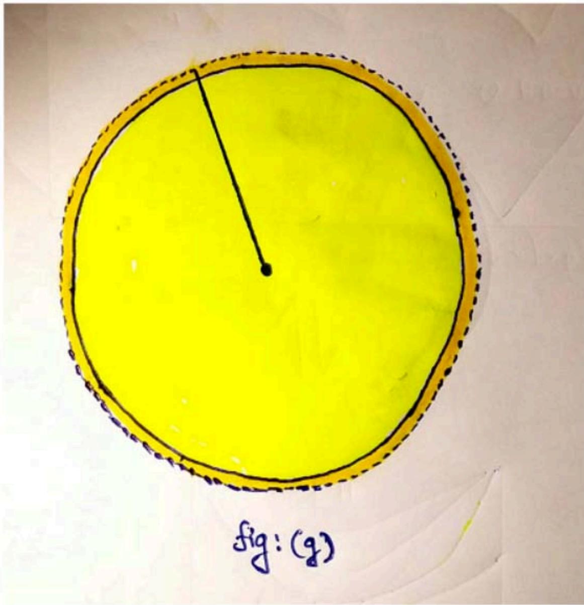So: $$ \begin{array}{l} DIAMETER = \operatorname{Log} (\text {Area}) \\ = \operatorname{Log} [ \exp (2 ^ {\mathrm {n}}) ] \\ = 2 ^ {\mathrm {n}} \\ \end{array} $$ So, that's the model of complexity geometry! Only other statements is that the identity operator is identified by the center of the disc (see fig: f). Now, what is the diameter of the geometry??? The diameter of this geometry is the distance from the origin (from the identity of the polygon); and it's not hard to see this corresponds to the logarithm of the area. Means diameter~2 $^{\text{n}}$ . And that's also indicate the largest complexity (The largest distance from the origin is: 2 $^{\text{n}}$ ! Now, concentrate on the next picture! This picture (see the figure: g) has a line that connect the origin (or, the identity) to the boundary! Suppose it represent a trajectory, in which the complexity increases. The point a(t): That's the moving point, moves out, we can think of it as: e^{-iHt}. There is an important point about geodesics and e^{-iHt}. In general geometry; e^{-iHt} actually generated a curve in geometry; but not necessarily a geodesic. It's only if it is both geodesic and killing direction both match with the thing generated by e^{-iHt}. So that's the important thing to know. Following a particular geodesic; generated by some Hamiltonian, and just following it out on this model for the complexity geometry, we can see it in terms of a series of unitary operators, but of course the geometry is simple to really represent that! $$ \mathrm {a (t) = e^{-i H t} = U (t)} $$ Complexity Grows Linearly.... (I.E Complexity Ramp) So, as you move from the origin the complexity grows linearly as you move the distance from the origin! It grows linearly with the parameter we are talking about could be the distance itself, and obviously the distance grow linearly with the complexity! So what that representing? That, representing the "complexity-ramp"! The linear growth of complexity as you move away from the reference state. So, that's first of all. 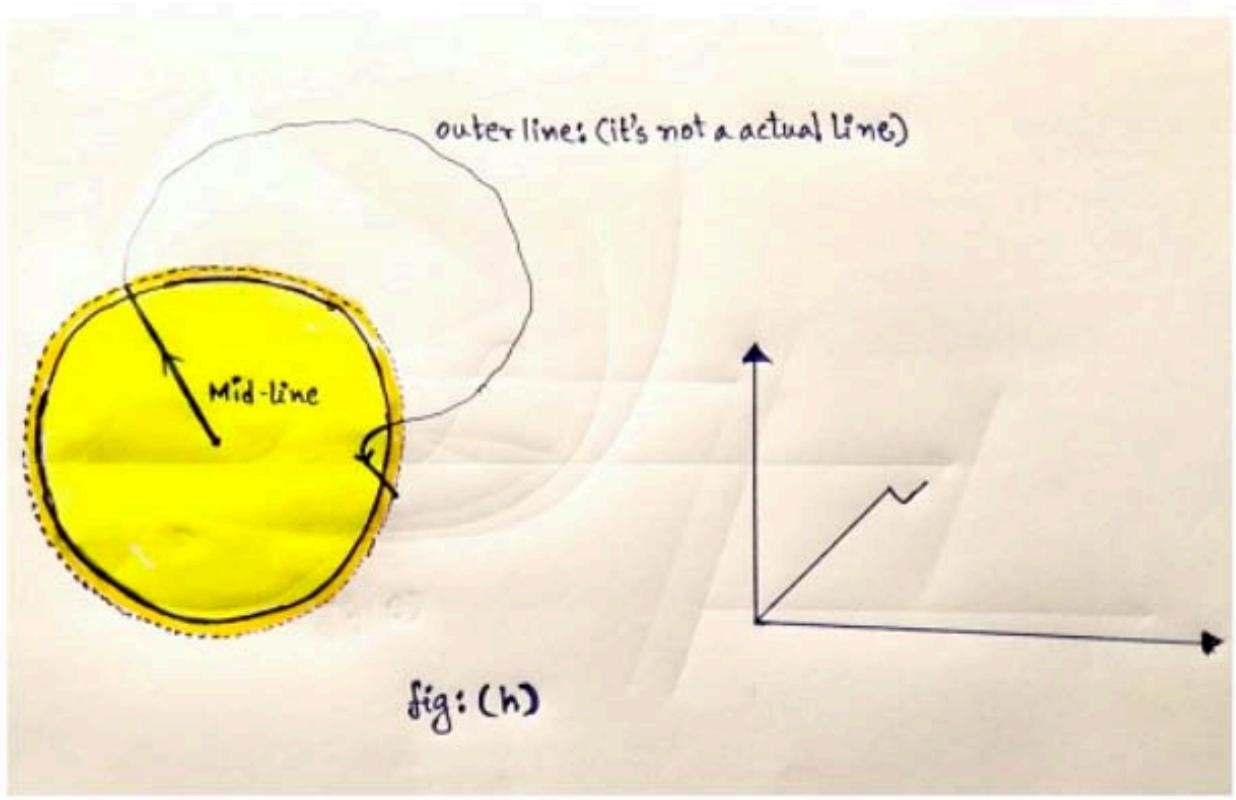And how long it's last? It last the diameter of the geometry, sometimes $\sim 2^{\mathrm{n}}$ . What happens next??? Now, we use random identifications. The next picture is the random identification (see the figure: h) of a particular point end of "Mid-line" with some other point or the other side of the polygon! So the "outer-line" just make sure to guide your eye. Actually there is no "outer-line" it just a jump! But strictly speaking, there actually no jump on the geometry either. It's just an identification! So let me called it a "Jump" (see the fig: h)! The jump across a new point. Where you reenter in the geometry; and since you out from the maximum distance, all you can do just go-in, a little bit. But because there are so many states; so many points out near the boundary; what tends to happen overwhelmingly probable that you not go very far!!! Just return to the polygon again. And there is double exponential probability for this to be happen. Means we won't get very far; just bounce around among the maximally complex states you like! If i plotted the growth of Complexity or the distance from the origin you would see the linear growth; you will get-up the polygon (i.e "outer line") and you will see in the graph that: complexity decreases for a short period of time and then sudden increases. Which i drawn in the figure here! Now, let's keep going! 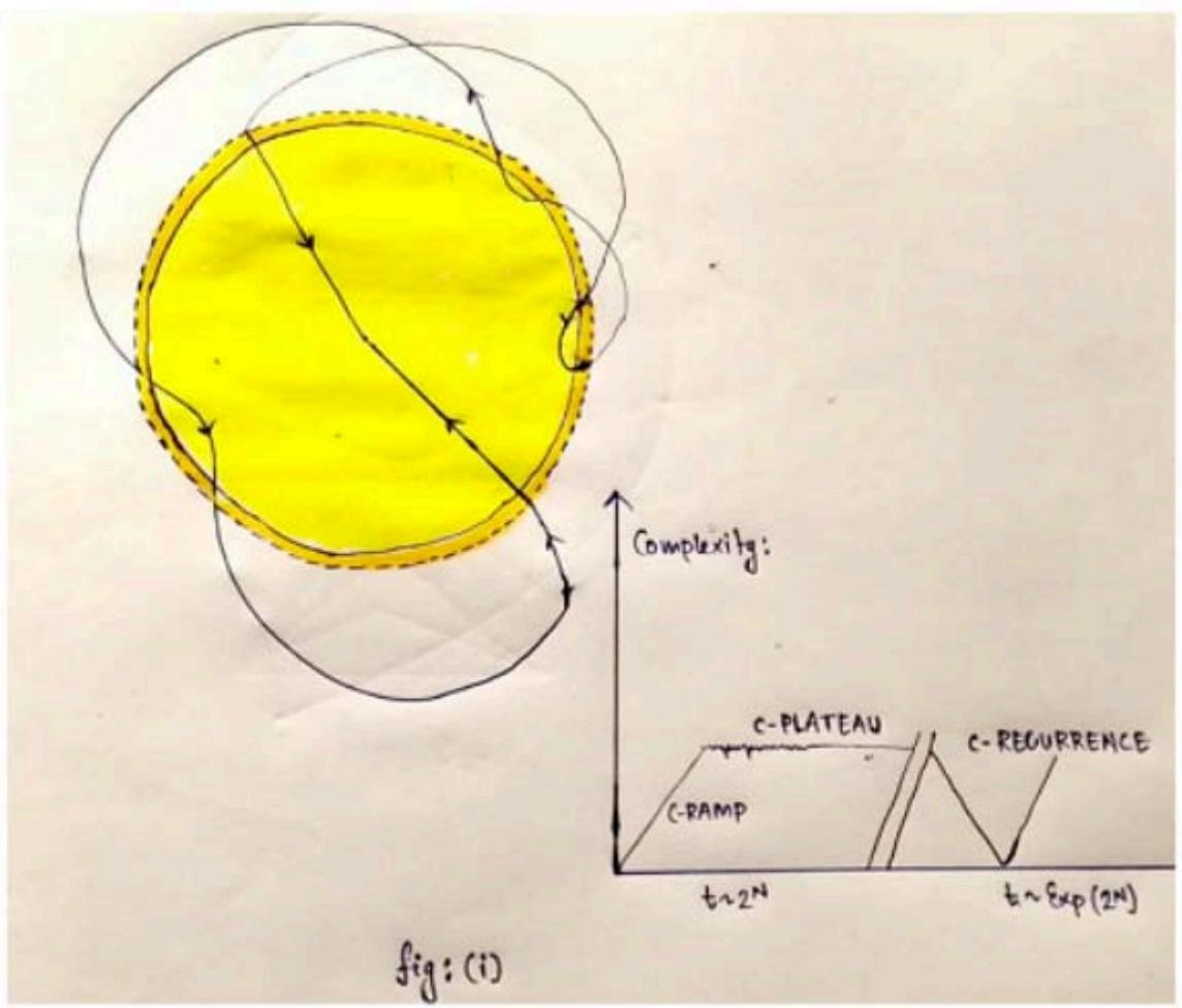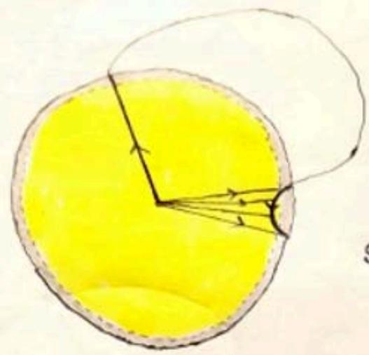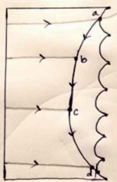In the next figure (see the figure: i) we go-out from the origin, we swing around, we hit the polygon, we jump to some new point, so what's actually happens??? Very quickly we exit the geometry again, go to some new point: go in, exit the geometry little bit, and so forth so on....! Almost endlessly (because there are so many points outside the boundary, that represents the maximum complex states; and you just bounce around them for exponential amount of time! But every once in a while by accident you are just happen to hit the polygon, just such a way; that you wind-up coming inward along a radial direction and get back to the origin or very close to the origin. That is "Quantum Recurrence". It takes double exponential amount of time. And just you can see; this model reproduces the "complexity-ramp", "complexity-plateau", and existence of very very infrequent "recurrence"! it's produce lot of other things about complexity, from which i get into now: "The Switch Back Effect"! Okay, now let's try to follow: "shortest-geodesic"! 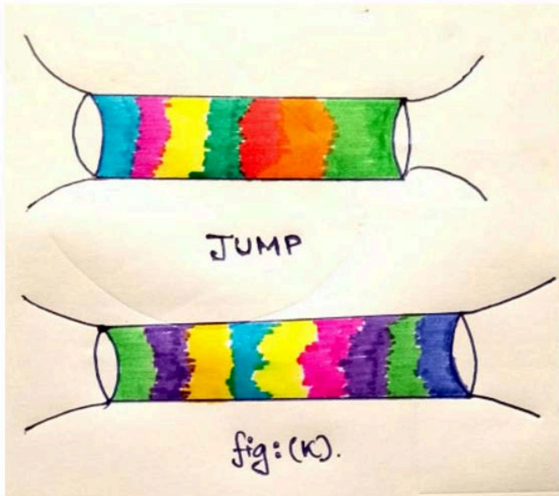The shortest geodesic (see the figure: j), once you get-out the polygon and make a jump, the shortest geodesic will also be jump. you will have to hit the cut-locus. You can see that from the picture (see the fig: j); once you re-enter the geometry, the geodesic (outer geodesic) longer than the inner-geodesics which connect the origin more directly with moving point a(t). In other words, the polygon is the "cut-locus" (see the fig: j). On other words at the point in which the transition of the "C-plateau" happens. In particular let's looked at the geodesics, once which are more direct and shorter than "outer-geodesics!" Those are also, be generated by a kind of Hamiltonian flow, but in general they are not the Hamiltonian flow's which are generated by a time independent Hamiltonian (or any curve on the geometry can be represented as a flow or Hamiltonian evolution as a time dependent Hamiltonian). And so the expectation (if you know little bit about this things) is that a typical geodesic is just drawn from the class of geodesics, will be something generated by a time dependent Hamiltonian. So when you get to the point "a", [just re-enter the geometry] the black curve generated by a Hamiltonian H_a. By the time you get to the point "b", another Hamiltonian will generate the curve, that's connect to the pont "b". By the time you get to the "c" a different Hamiltonian connect the point "c". And finally you get to the "d", you get a different one. What's going on actually??? I claim that the worm-hole or the evolution of the worm-hole is continuously changing [Is being generated instead of by a time-dependent hamiltonian; by a sequence of time dependent hamiltonian] between the point "a" and "d"! But then what happen when you get to the point "d" (see the fig: j)! When you get to the point "d", you get to the boundary again and you jump to some place else; a discontinuous transition happens, and that discontinuous transition means, the length of the geodesics doesn't change, but the whole character of the hamiltonian which generates it [The whole internal structure of it], will change discontinuously! This discontinuous changes (short time interval of continuous change), they are generated noise on the top of the complexity curve)! So what it say about worm-holes??? It Say's, as you make one of this jumps the whole internal structure of the worm-hole changes! Not in length; but the internal structure; you might think it in terms of "Tensor Networks", so the character of the Tensor networks jump from one tensor network to another! And if it's true, the hamiltonian which generate this flows is must time dependent. And that translate into the worm-hole is inhomogeneous. It's generated in a way which is dependent on way you are in worm-hole. And what it should do; it creates an inhomogeneous behavior to the worm-hole! In other way to say it; the worm-hole probably full of matter, with an inhomogeneous structure to it (see the figure: k)! When you get that point, suddenly the worm-hole become an inhomogeneous thing or stuff, it shrink little bit and, then grows back (C-plateau)! And then make's another jump (it makes another discontinuous jump)! After it makes another discontinuous jump it evolve a little bit continuously and then jump again and jump again. So what I'm guessing: the post exponential time (after the exponential time), the worm-hole have a geometry, it's full of inhomogeneous matter! And theorist Henry.Lin Called it as a "Caterpillars"! Why a Caterpillar?? Because, it's long and segmented! But I think the word "caterpillar" is more technical on this context! That's I'm expecting the Interior of the black-hole to look like, after an exponential of time. I think it has a geometry, and the geometry might be reasonably smooth but it could different the kind of geometry we expect in early times! Let me do some summarization of thoughts! There are three descriptions that i given you! i. "You just keep growing theory": That really worm-holes don't have to do with complexity! They just keep growing and growing. And this theory known as: "pseudo-complexity"! I don't think it wrong. I think it's answers are some particular questions! Q: How many gates did the natural evolution of the black-hole use to arrive at some Quantum state: $|\Psi (t)\rangle \coloneqq \dots$ ii. Quantum superposition of sub-exponential states! That's the picture, where you go beyond exponential, you run out of states! Behavior of the clock (instead of registering a coherent time), just grows into a state of superposition of all possible time!!! I think, that's a correct description. Mainly for the boundary description (The Quantum Mechanical Boundary Description), of the measurable things in the black-hole. iii. Finally, the minimal geodesic description! The shortest circuit, or the shortest Tensor networks they all are the same thing! So the shortest geodesic; that the picture "caterpillar" picture! But what the question does it answer??? Q: It answer the question what is the minimal number of gates needed to shrink the worm-hole back to the reference state! (Reference state: very short worm-hole, or in terms of complexity it has almost zero complexity)! 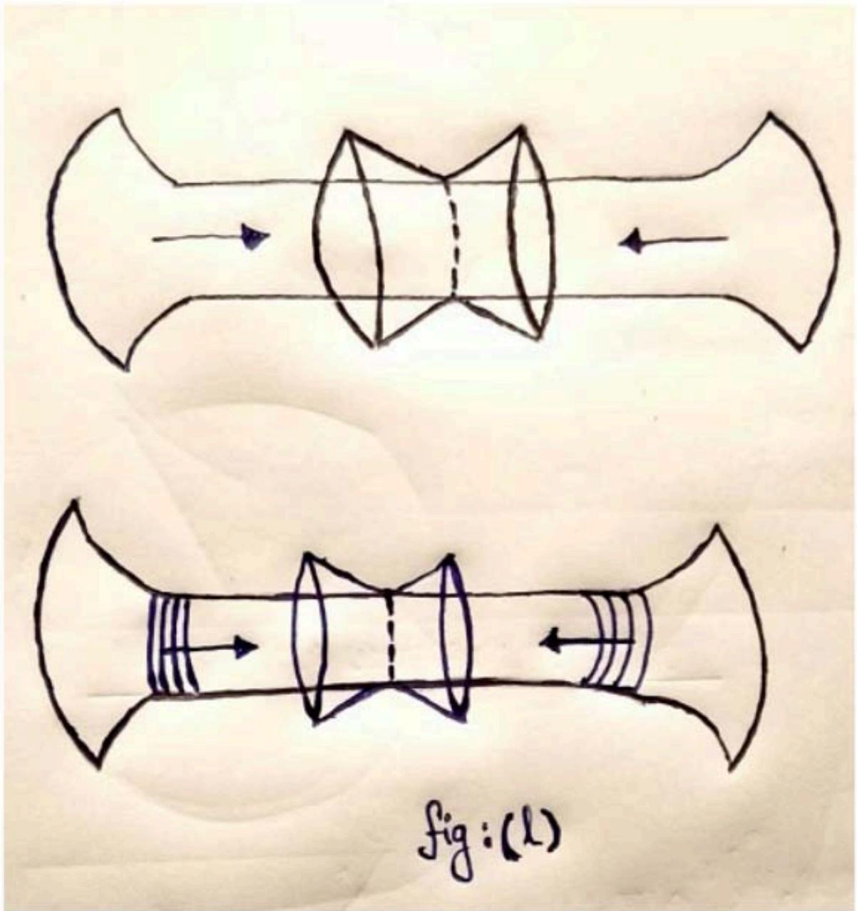How you shorten worm-hole??? You may apply operations at the end and those operations simply decreases the size of the worm-hole from the boundary or from the horizon inwards! What is the minimum number of gates [not the number that if you time reverse the natural evolution] could possibly bring you back to the simple state??? That are the three different questions; with three different answers!!! (See the fig: l) But the remarkable thing is that; in sub-exponential time; this three description are same! We can come back to that! But the post exponential time, the three different description are different. I mean: "The Keep Growing Theory", "The Quantum Superposition", and "shortest-geodesic"! Okay, now which one is right??? Yes, some sense they all right! But, they answer different questions! (a) So, let's start with "Just Keep Growing Theory" or "JKGT!" The "JKGT" gives absurd results. In certain sense absurd. You can see the absurdity must clear if you go to the "Quantum Recurrence"! If you go to a "Quantum Recurrence", the state returns into the simplest possible state! Namely the "TFD" or "Thermal Field Double!" And in TFD, the measurable entities, the correlations between the field on the left side and right side goes to large! Characteristics of a worm-hole is very short in size! Now if you jumped back into quantum recurrence, (close to the thermal field double), you may see: the Alice-Bob experiment is succeeded. So what is the Alice-Bob experiment??? Alice jumped into her side, Bob into his side, and they meet in the middle! But that won't happen if the worm-hole is very long. As they meet in a traversable experiment, so that's the reason it called "Traversable worm-hole"! And in every possible way, the state of the black-hole is the Short worm-hole. But if you consider the "Keep Growing Theory: the volume and the length of the worm-hole increases exponentially! So, the "JKGT" or "Pseudo-complexity" doesn't make any reasonable description between what happens inside and what type of correlation acour in the boundary (or B·H—W·H side)!!! (b) Now, what about the linear superposition theory???? "LST"—i think it's right. It's answers are right but it actually gives nothing about the character of the interior. The reason i say that: (i) Because, the mapping or the dictionary between boundary and the Interior of the black-hole is itself enormously complex! Because the bulk properties of the interior are connected with the boundary quantum mechanics by an insane complicated map, which some how random in nature! Or, atleast pseudo-random. Another reason is that, the linearity of superposition of states in the boundary theory, doesn't transform into the linearity of superposition of states in the bulk theory. 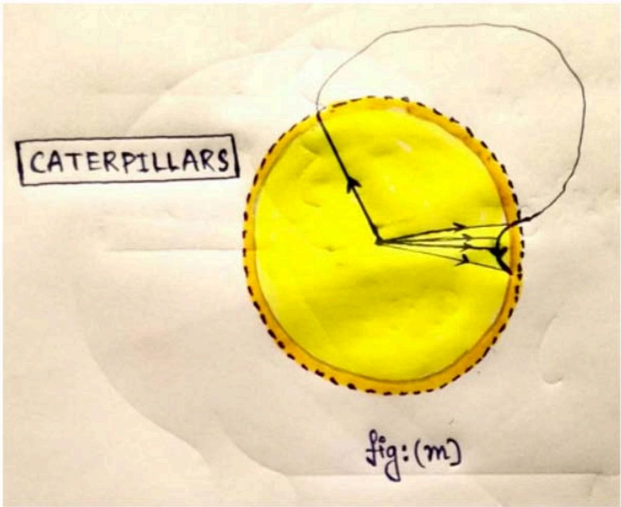(C) What about the 3rd option??? The worm-hole geometry is governed by the minimal circuit/gates; minimal geodesics; minimal tensor network; that as far as i can tell; is consistent with all measurable probes (even those designed to probe the Interior)! And gives rise to a picture (see the fig: m) which is geometric but unusual compared to how the wormhole evolves! And i think it's the only one; which gives rise to the reasonably geometric picture of the Interior! # III. CONCLUSION So finally what I get? I get an overview here! Here is the "History Of Complexity"! And if you believe in "complexity-volume" connection [The volume of the "wormhole"!]; long long periods of complexity equilibrium double exponential, where the black hole sits most complex kinds of states, with the worm-hole just single exponential long fluctuations can change its character, from instant to instant But yes, it's punctuated by Boltzmann type complexity fluctuations. By Boltzmann type complexity fluctuations, I mean: quantum mechanical recurrence [partial recurrence or even full recurrences] they are exceedingly rare! But it's only during those complexity recurrences, the classical General Relativity describe the interior! So only doing complete recurrences, this penrose diagram describes what's going on! In other words, the penrose diagram itself is a description of recurrence [see Fig. n]         Shortest Geodesic TRANSITION FROM: Dark blue to blue! Let's blow up that lil bit!  $$ Te ^{- i \int_{0}^{a} H_{a} (t^{\prime}) d t^{\prime}}; $$ $$ Te ^{- i \int_{0}^{b} H_{u} (t) \cdot d t^{\prime}}; $$ $$ Te ^{- i \int_{0}^{c} H_{c} (t^{\prime}) d t^{\prime}}; $$ $$ Te ^{- i \int_{0}^{d} H_{d} (t) d t}; $$ Fig: (j)     $$ \downharpoonleft \upharpoonright $$  Describe The Interior Fig: (n)

Generating HTML Viewer...