I. INTRODUCTION
II. PRELIMINARIES
Consider the Erlang risk model (2) that is perturbed by Brownian motion:
\[U(t) = u + c t + \sigma B(t) - \sum_{i=1}^{N(t)} X_i,\]
where
-
is the initial capital and c is the constant rate of premium per unit of time,
-
, the number of claim occurrences is described by a renewal process,
-
, sequence of strictly positive random variables, i.i.d., independent of is the amount of the i-th claim. represents their distribution function, the density function and the Laplace transform.
-
, standard Brownian motion is independent of , i.e. independent of and .
-
is the diffusion volatility.
Let , be the inter-occurrence times of the claim, that is a sequence of strictly positive random variables and i.i.d. having an Erlang distribution (2) of parameter with being the time of occurrence of the th claim throughout our investigations. represents their distribution function, the density function and the Laplace transform such that:
\[f_{V}(t) = \lambda^{2} t e^{-\lambda t},\]
\[F_{V}(t) = 1 - e^{-\lambda t} - \lambda t e^{-\lambda t},\]
\[f _ {V} ^ {*} (s) = \mathbb {E} \left[ e ^ {- s V} \right] = \left(\frac {\lambda}{\lambda + s}\right) ^ {2}.\tag{4}\]
We also assume that X has an Erlang (2) distribution with parameter and that the form a sequence of random vectors i.i.d. as the canonical vector with the possibility that the components of such a vector are dependent.
Finally, we assume that the claim amounts are exponentially distributed with a parameter , that the random vectors claim amounts and interclaim occurrence times is a sequence of random variables with the same distribution as the random vector .
We denote the joint cumulative distribution function of the distribution function of claim amounts and interclaim occurrence times where .
The moment of ruin , which is the first time the risk process reaches a negative value associated with the risk model (1), is written as follows:
\[\tau = \left\{ \begin{array}{c} \inf \left\{t \geq 0: U (t) < 0 \mid U (0) = u \right\} \\ \infty \quad \text {si} U (t) \geq 0, \forall t \geq 0. \end{array} \right.\tag{5}\]
The probability of ruin in finite time t is defined as follows:
\[\psi (u) = \mathbb {P} \left(\tau \in [ 0, t ], U (t) < 0 \mid U (0) = u\right),\]
and the probability of ultimate ruin (infinite-horizon probability) by:
\[\psi (u) = \psi (u, \infty) = \mathbb {P} (\tau < \infty , U (t) < 0 \mid U (0) = u).\]
We decompose the probability of ruin as in [12] by:
\[\psi (u) = \psi_ {w} (u) + \psi_ {d} (u).\tag{6}\]
This decomposition is justified by the fact that the probability of ruin can be caused either by the claim amounts , or by the oscillation of the Brownian motion . To ensure that ruin is not a certain event, we assume that net profit satisfies the following inequality:
\[\mathbb{E}\left[cV-X\right]>0.\]
We can verify by rigorous calculations that (7) is equivalent to:
\[c \beta^ {2} > \lambda^ {2}.\]
In order to better study ruin measures, we introduce the Gerber-Shiu function defined by:
\[\phi(u) = \mathbb{E}\left[ e^{-\delta\tau} \omega\left(U(\tau^{-}), |U(\tau)|\right) I(\tau < \infty) \,|\, U(0) = u \right]\]
where is the force of interest; is the indicator function; , the non-negative value of the penalty function is a function of the surplus just before bankruptcy and the deficit at bankruptcy for . So is the probability of ruin, the Gerber-Shiu function can be broken down according to whether the ruin is caused by the claim amounts or by the oscillation, i.e:
\[\phi (u) = \phi_ {w} (u) + \phi_ {d} (u),\tag{9}\]
where
\[\phi_ {w} (u) = \mathbb {E} \left[ e ^ {- \delta \tau} \omega (U (\tau^ {-}), | U (\tau) |) I (\tau < \infty , U (t) < 0) | U (0) = u \right],\tag{10}\]
is the Gerber-Shiu function when ruin is generated by claim amounts, and
\[\begin{array}{r c l} \phi_ {d} (u) & = & \mathbb {E} \left[ e ^ {- \delta \tau} \omega (U (\tau^ {-}), | U (\tau) |) I (\tau < \infty , U (t) = 0) | U (0) = u \right] \\& = & \omega (0, 0) \mathbb {E} \left[ e ^ {- \delta \tau} I (\tau < \infty , U (t) = 0) | U (0) = u \right], \end{array}\tag{11}\]
is the Gerber-Shiu function when the ruin is generated by the oscillation of Brownian motion. For simplicity, we assume that . We also note that a particular parameterisation of and brings and to the probabilities of ruin and .
2.1 Dependency structure
The concept of copula was introduced in 1959 by Abe Sklar. The copula are functions that provides a general framework for studying associated structures of random variables and constructing multivariate distribution function using univariate marginal functions and multivariate correlation structure functions. Copulas are used extensively to model the structure of dependence between multiple random variables in finance and insurance ([15],[16],[17],[18])
2.1.1 Tail dependence
Tail dependence is a measure of comovements in the tails of a bivariate distributions. He describes the describe the level of dependence at the extremes of the distribution. Tail dependence represents the limiting proportion that one margin exceeds a certain threshold given that the other mzrgin hzd already exceeded that threshold. This measure is of great importance for extreme events. There are two tail dependence coefficients (upper tail dependence and lower tail dependence) which are defined as follows:
Definition 2.1 Let X; Y two continuous random variables with respective distribution functions F and G. The lower tail dependence coefficient is defined by:
\[\lambda_ {L} (X, Y) = \lim _ {\alpha \rightarrow 0 ^ {+}} \mathbb {P} \left(X \leq F ^ {- 1} (\alpha) \mid Y \leq G ^ {- 1} (\alpha)\right)\tag{12}\]
and the upper tail dependence coefficient is defined by:
\[\lambda_ {U} (X, Y) = \lim _ {\alpha \to 1 ^ {-}} \mathbb {P} \left(X > F ^ {- 1} (\alpha) \mid Y > G ^ {- 1} (\alpha)\right)\]
These measurements can be defined in terms of a copula C.
Definition 2.2 (Tail dependence) Let X; Y be two continuous random variables of copula C, then we have
\[\lambda_ {L} (X, Y) = \lim _ {u \to 0 ^ {+}} \frac{C (u , u)}{u} \quad and \quad \lambda_ {U} (X, Y) = \lim _ {u \to 1 ^ {-}} \frac{1 - 2 u + C (u , u)}{1 - u}.\]
Remark 2.1
-
When ; then has a lower tail dependency.
-
When ; then has no lower tail dependency.
-
When ; then has an upper tail dependency.
-
When ; then has no upper tail dependency
Many authors ([11], [12], [9], [19]) have used the Farlie-Gumbel-Morgenstern (FGM) copula to define the dependency structure between the claim sizes and interclaim times. The FGM copula is given by:
\[C _ {\alpha} (u, v) = u v + \alpha u v (1 - u) (1 - v); 0 \leq u, v \leq 1.\tag{13}\]
It is not suitable for modelling dependencies on extreme values because .
2.1.2 Dependency model based on Spearman's copula
In this article, the dependency structure of the random vector of the amounts of claims and the inter-occurrence times of the claims is described with a copula . In particular, we use the linear Spearman copula studied in [15] then in [14] and defined in [16] by:
\[\forall \alpha \in [ 0, 1 ], \forall (u, v) \in [ 0, 1 ] ^ {2}, C _ {\alpha} (u, v) = (1 - \alpha) C _ {I} (u, v) + \alpha C _ {M} (u, v),\tag{14}\]
where
\[C_{I}(u,v)=uv\quad\text{and}\quad C_{M}(u,v)=\min(u,v).\]
The parameter represents the degree of dependency.
The Spearman copula admits interesting properties in cases with extreme values. Indeed, it suitable for modeling rare events in finance and insurance (earthquakes, hurricanes, floods, etc.) because its upper tail dependence coefficient is equal to its degree of dependence, .
The bivariate distribution function F of claim amounts and claim inter-occurrence times with margins and can be written as (For the interested reader, see [17]).
The Spearman copula is a convex combination of the independent copula and the comonotone copula (positive dependence between the components of the random vector). This copula also has the ability to capture tail dependence in many situations such as earthquakes and other rare events ([18], [20]).
The Spearman copula is given by , we obtain:
\[\begin{array}{r c l} F (x, t) & = & C _ {\alpha} \left(F _ {X} (x), F _ {V} (t)\right) \\& = & (1 - \alpha) C _ {I} \left(F _ {X} (x), F _ {V} (t)\right) + \alpha C _ {M} \left(F _ {X} (x), F _ {V} (t)\right) \\& = & (1 - \alpha) F _ {I} (x, t) + \alpha F _ {M} (x, t). \end{array}\tag{15}\]
The copula on , has the set as support. Furthermore, on and is the uniform distribution on . When the dependent structure of is described by the copula , then they are comonotones and there almost certainly exists an increasing function , such that (See [17]). The distribution function of then satisfies:
\[F _ {X} (x) = F _ {V} \left(l ^ {- 1} (x)\right) \Longleftrightarrow 1 - e ^ {- \beta x} - \beta t e ^ {- \beta x} = 1 - e ^ {- \lambda l ^ {- 1} (x)} - \lambda l ^ {- 1} (x) e ^ {- \lambda l ^ {- 1} (x)}.\]
First of all, we note by identification that
\[e ^ {- \beta x} (1 + \beta t) = e ^ {- \lambda l ^ {- 1} (x)} (1 + \lambda l ^ {- 1} (x))\]
then by a suitable deduction
\[\beta t = \lambda l ^ {- 1} (x)\]
and last but not least
\[l^{-1}(x) = \frac{\beta t}{\lambda}\]
This gives us
\[\frac {1}{\beta} = \int_ {0} ^ {\infty} e ^ {- \lambda l ^ {- 1} (x)} d x.\tag{17}\]
From (16), we have . The joint distribution of the random vector is singular on the set as support. Similarly, it is the distribution on .
2.1.2 Dependency model based on Spearman's copula
In this subsection, we analyse the solutions of the Lundberg-type equation associated with the risk model (1) and we determine the Laplace transforms of the Gerber-Shiu functions. The Laplace transform of a function is denoted .
By , we denote the arrival time of the -th claim with .
Let's assume that and , , the surplus immediately after the -th claim takes the form:
\[\begin{array}{r c l} U _ {n} = U \left(T _ {n}\right) & = & u + c T _ {n} + \sigma B \left(T _ {n}\right) - \sum_ {i = 1} ^ {n} X _ {i} \\& = & u + \sum_ {i = 1} ^ {n} \left[ c V _ {i} + \sigma B \left(V _ {i}\right) - X _ {i} \right]. \end{array}\]
This last equality can be written as in [12], that is:
\[\begin{array}{r c l} U _ {n} & \stackrel {{D}} {{=}} & u + \sum_ {i = 1} ^ {n} (c V _ {i} - X _ {i}) + \sigma B \bigg (\sum_ {i = 1} ^ {n} V _ {i} \bigg) \\& \stackrel {{D}} {{=}} & u + \sum_ {i = 1} ^ {n} (c V _ {i} - X _ {i} + \sigma B (V _ {i})) , \end{array}\]
where means "equality in distribution".
Consequently, the equation (1) can take the following form:
\[U \left(\sum_ {i = 1} ^ {n} V _ {i}\right) = u + \sum_ {i = 1} ^ {n} \left(c V _ {i} - X _ {i} + \sigma B \left(V _ {i}\right)\right).\]
We adopt the "martingale" approach to determine the ruin time of the force of interest . Since the claim amounts are distributed exponentially, we have a light-tailed distribution, hence the adjustment coefficient noted , also known as the Lundberg exponent.
To determine the number such that the process is a martingale, we:
-
first use the Lundberg inequality given in [21], theorem 2.1 on page 63 which guarantees that the probability of ultimate ruin satisfies the inequality with ,
-
then increase this probability of failure by introducing an exponential martingale from theorem 2.1 of [22], page 322,
-
finally deduce the adjustment coefficient as in [7] with , which satisfies the following equation in our case
\[\mathbb {E} \left[ e ^ {- s (c V - X + \sigma B (V))} \right] = 1.\tag{18}\]
The equation is called the Lundberg-type equation associated with the risk model. We shall see that it is essential for ruin measures.
We note that with (15), the equation (18) is written in the form (See [13]):
\[(1 - \alpha) J _ {I} + \alpha J _ {M},\tag{19}\]
\[J_{I} = \frac{\lambda^{2} \beta^{2}}{(\beta + s)^{2} \left(\lambda + \delta - \frac{\sigma^{2}}{2} s^{2} - c s\right)^{2}}\]
with the real part of the number denoted , positive and . What's more
\[J_{M} = \frac{\lambda^{2}\beta^{2}}{\left(-\frac{\sigma^{2}}{2}\beta s^{2} - (c\beta - \lambda) s + (\delta + \lambda) \beta\right)^{2}}\]
with the real part , positive and .
Lemma 2.1
i. When and , the generalised Lundberg equation (18) has exactly two solutions noted , with , .
ii. When , the equation (18) has exactly one solution noted , with and a second solution .
Proof. We start with i and end with ii.
being the Laplace transform of an exponential distribution exponential with parameter , we have . In addition, we have . While observing the lemma 3.1 in [13], we obtain without difficulty
\[J _ {I} = \frac {\lambda^ {2} \beta^ {2}}{(\lambda + \delta - s c - \frac {\sigma^ {2}}{2} s ^ {2}) ^ {2} (s + \beta) ^ {2}} \quad \text {and} \quad J _ {M} = \frac {\lambda^ {2} \beta^ {2}}{\left(- \frac {1}{2} \sigma^ {2} \beta s ^ {2} + (\lambda - c \beta) s + \beta (\lambda + \delta)\right) ^ {2}}\tag{22}\]
with , and . In this case, the equation (18) can be written as
\[\frac{\lambda^{2} \beta^{2} (1 - \alpha)}{(\lambda + \delta - s c - \frac{\sigma^{2}}{2} s^{2}) ^ {2} (s + \beta) ^ {2}} + \frac{\lambda^{2} \beta^{2} \alpha}{\left(- \frac{1}{2} \sigma^{2} \beta s^{2} + (\lambda - c \beta) s + (\beta \lambda + \beta \delta)\right) ^ {2}} = 1\]
with and .
When , the equation (23) coincides with equation (2.19) in [23].
For , the equation (23) is equivalent to:
\[h _ {1} (s) = h _ {2} (s),\tag{24}\]
\[h _ {1} (s) = (\beta + s) ^ {2} \left(\lambda + \delta - \frac {\sigma^ {2}}{2} s ^ {2} - c s\right) ^ {2} \left(- \frac {\sigma^ {2}}{2} \beta s ^ {2} - (c \beta - \lambda) s + (\delta + \lambda) \beta\right) ^ {2}\]
\[h _ {2} (s) = (1 - \alpha) \lambda^ {2} \beta^ {2} \left(- \frac{\sigma^ {2}}{2} \beta s ^ {2} - (c \beta - \lambda) s + (\delta + \lambda) \beta\right) ^ {2} + \alpha \lambda^ {2} \beta^ {2} (\beta + s) ^ {2} \left(\lambda + \delta - \frac{\sigma^ {2}}{2} s ^ {2} - c s\right) ^ {2}.\]
By applying Rouche's theorem [24] to the closed contour as in [13], we have:
\[\lim _ {s \to \infty} \left| \frac {\lambda^ {2} \beta^ {2} (1 - \alpha)}{(\lambda + \delta - s c - \frac {\sigma^ {2}}{2} s ^ {2}) ^ {2} (s + \beta) ^ {2}} + \frac {\lambda^ {2} \beta^ {2} \alpha}{(- \frac {\sigma^ {2}}{2} \beta s ^ {2} + (\lambda - c \beta) s + \beta (\lambda + \delta)) ^ {2}} \right| = 0\tag{25}\]
on the contour C where .
Furthermore, for , we can see that:
\[\frac {(1 - \alpha) \lambda^ {2} \beta^ {2}}{(\beta + s) ^ {2} \left(\lambda + \delta - \frac {\sigma^ {2}}{2} s ^ {2} - c s\right) ^ {2}} \quad \text {and} \quad \frac {\alpha \lambda^ {2} \beta^ {2}}{\left(- \frac {\sigma^ {2}}{2} \beta s ^ {2} - (c \beta - \lambda) s + (\delta + \lambda) \beta\right) ^ {2}} > 0.\tag{26}\]
Also, for and , we have
\[\frac {\lambda^ {2} \beta^ {2} (1 - \alpha)}{\beta^ {2} (\lambda + \delta) ^ {2}} + \frac {\lambda^ {2} \beta^ {2} \alpha}{(\beta \lambda + \beta \delta) ^ {2}} = \left(\frac {\lambda \beta}{\beta (\lambda + \delta)}\right) ^ {2} < 1,\tag{27}\]
because
Finally, by posing
\[q (s) = \left| \frac {\lambda^ {2} \beta^ {2} (1 - \alpha)}{(\lambda + \delta - s c - \frac {\sigma^ {2}}{2} s ^ {2}) ^ {2} (s + \beta) ^ {2}} + \frac {\lambda^ {2} \beta^ {2} \alpha}{\left(- \frac {1}{2} \sigma^ {2} \beta s ^ {2} + (\lambda - c \beta) s + \beta (\lambda + \delta)\right) ^ {2}} \right|,\]
we have:
\[\begin{array}{r c l} q (s) & \leq & \left| \frac {\lambda^ {2} \beta^ {2} (1 - \alpha)}{(\lambda + \delta - s c - \frac {\sigma^ {2}}{2} s ^ {2}) ^ {2} (s + \beta) ^ {2}} \right| + \left| \frac {\lambda^ {2} \beta^ {2} \alpha}{(- \frac {1}{2} \sigma^ {2} \beta s ^ {2} + (\lambda - c \beta) s + \beta (\lambda + \delta)) ^ {2}} \right| \\& \leq & \frac {\lambda^ {2} \beta^ {2} (1 - \alpha)}{\beta^ {2} (\lambda + \delta) ^ {2}} + \frac {\lambda^ {2} \beta^ {2} \alpha}{\beta (\lambda + \delta) ^ {2}} \\& \leq & 1. \end{array}\tag{28}\]
Since has exactly two zeros inside the contour , by application of Rouche's theorem, also has two zeros inside the contour noted , with , .
For , the conditions of Rouche's theorem are not satisfied because
\[\left| \frac {\lambda^ {2} \beta^ {2} (1 - \alpha)}{(\lambda + \delta - s c - \frac {\sigma^ {2}}{2} s ^ {2}) ^ {2} (s + \beta) ^ {2}} + \frac {\lambda^ {2} \beta^ {2} \alpha}{(- \frac {1}{2} \sigma^ {2} \beta s ^ {2} + (\lambda - c \beta) s + (\beta \lambda + \beta \delta)) ^ {2}} \right| = 1\tag{29}\]
for . The proof ii. can be obtained by using an extension of Rouch ©'s theorem, called Klimenok's theorem in [25].
Remark 2.2 For , the equation (18) has at least one positive real root denoted by . is a polynomial with exactly two positive zeros noted:
\[s_1 = -\frac{1}{\sigma^2} \left(c - \sqrt{2 (\lambda + \delta) \sigma^2 + c^2}\right),\]
\[s _ {2} = \frac {1}{\sigma^ {2} \beta} \left(\lambda - c \beta + \sqrt {(\lambda - c \beta) ^ {2} + 2 (\lambda + \delta) \beta^ {2} \sigma^ {2}}\right).\tag{31}\]
It is immediately clear that .
Let's calculate and
\[h _ {2} (0) = \lambda^ {2} \beta^ {4} (\lambda + \delta) ^ {2} \leq \beta^ {4} (\lambda + \delta) ^ {4} = h _ {1} (0).\]
\[\begin{array}{r l} h _ {2} (s _ {1}) = & (1 - \alpha) \lambda^ {2} \beta^ {2} \left(- \frac{\sigma^ {2}}{2} \beta s _ {1} ^ {2} - (c \beta - \lambda) s _ {1} + (\delta + \lambda) \beta\right) ^ {2} + \alpha \lambda^ {2} \beta^ {2} (\beta + s _ {1}) ^ {2} \biggl (\lambda + \delta - \frac{\sigma^ {2}}{2} s _ {1} ^ {2} - c s _ {1} \biggr) ^ {2} \\= & (1 - \alpha) \lambda^ {2} \beta^ {2} \biggl [ \beta \left(- \frac{\sigma^ {2}}{2} s _ {1} ^ {2} - c s _ {1} + \delta + \lambda\right) + \lambda s _ {1} \biggr ] ^ {2} \\= & (1 - \alpha) \lambda^ {4} \beta^ {4} s _ {1} ^ {2} \\> & 0 = h _ {1} (s _ {1}). \end{array}\]
Since and , we deduce by the intermediate value theorem that the equation (18) has a root satisfying .
Assume root is real. We have
\[h_{2}(s_1) = (1 - \alpha) \lambda^{4} \beta^{4} s_{1}^{2} > 0 = h_{1}(s_1).\]
\[\begin{array}{c} h _ {2} (s _ {2} = \left((1 - \alpha) \lambda^ {2} \beta^ {2} - \frac {\sigma^ {2}}{2} \beta s _ {2} ^ {2} - (c \beta - \lambda) s _ {2} + (\delta + \lambda) \beta\right) ^ {2} + \alpha \lambda^ {2} \beta^ {2} (\beta + s _ {2}) ^ {2} \left(\lambda + \delta - \frac {\sigma^ {2}}{2} s _ {2} ^ {2} - c s _ {2}\right) ^ {2} \\\alpha \lambda^ {2} \beta^ {2} (\beta + s _ {2}) ^ {2} \left(\lambda + \delta - \frac {\sigma^ {2}}{2} s _ {2} ^ {2} - c s _ {2}\right) ^ {2} \end{array}\]
\[= \alpha\lambda^{2}\beta^{2}(\beta+s_{2})^{2} \left[ \frac{1}{\beta} \left(-\frac{\sigma^{2}}{2}\beta s_{2}^{2}-c\beta s_{2}+\beta(\lambda+\delta)+\lambda s_{2}-\lambda s_{2}\right) \right]^{2}\]
We cannot conclude that is a real root.
III. MAIN RESULTS
In this section, we present the main results of the article.
3.1 Calculation of the ultimate probability of ruin due to claims
In this subsection, we determine the infinite-horizon probability of ruin when it is due to claims
Theorem 3.1 The ultimate probability of ruin due to a claim is given
\[\psi_ {w} (u) = \frac {2 \lambda a}{\beta (a ^ {2} \sigma^ {2} - a b \sigma^ {2})} \cdot e ^ {a u} + \frac {2 \lambda b}{\beta (b ^ {2} \sigma^ {2} - a b \sigma^ {2})} \cdot e ^ {b u}; u \geq 0\]
where
\[a = - \frac{1}{2 \sigma^{2}} \left(2 c + \sqrt{\sigma^{4} \beta^{2} + 8 \sigma^{2} \lambda + 4 c^{2} - 4 c \sigma^{2} \beta} + \sigma^{2} \beta\right) < 0\]
and
\[b = - \frac{1}{\sigma^{2}} \left(c - \frac{1}{2} \sqrt{\sigma^{4} \beta^{2} + 8 \sigma^{2} \lambda + 4 c^{2} - 4 c \sigma^{2} \beta} + \frac{1}{2} \sigma^{2} \beta\right) < 0.\]
To prove the theorem (3.1), we introduce some useful basic results and consider the lemmas (3.1), (3.2) and (3.3).
Let be an auxiliary function, a Brownian motion starting at 0 with -c drift and as variance. We denote the supremum of in the interval and , the first time of reaching the value u > 0. By Borrodin and Salminen's formula [26], we can obtain for ,
\[\mathbb {E} \left[ e ^ {- \delta \tau_ {u}} \right] = e ^ {- \eta u},\tag{32}\]
where
\[\eta = \frac{c}{\sigma^{2}} + \sqrt{\frac{2\delta}{\sigma^{2}} + \frac{c^{2}}{\sigma^{4}}}\]
For , we define the following potential measure:
\[\mathcal{P}(u,dx,dy) = \mathbb{E}\left[e^{-\delta V} I(\overline{W}(V) < u, W(V) \in dy, X \in dx)\right], \quad u,x > 0, \quad y < u.\]
We denote by , an exponential random variable of rate q. We can therefore first calculate the following measure:
\[\mathcal{U}_{q}(u,dy) = \operatorname{Pr}\left(\overline{W}(e_{q}) < u, W(e_{q}) \in dy,\right), \quad u > 0, \quad u > y.\]
which can be obtained by the lemma of [27], well known in applied probability.
Finally, we denote by: and , the differentiation operators and I the identity operator with the differentiation operator A defined as follows:
\[A (\mathcal {D}) = \mathcal {D} ^ {2} + \frac {2 c}{\sigma^ {2}} \mathcal {D} - \frac {2 (\lambda + \delta)}{\sigma^ {2}} \mathcal {I}.\tag{34}\]
Furthermore, it is easy to notice that:
\[A\left(\mathcal{D}\right) = \left(\mathcal{D} + \eta_{1} \mathcal{I}\right) \left(\mathcal{D} - \eta_{2} \mathcal{I}\right).\]
Lemma 3.1 For u > 0, the Gerber-Shiu function satisfies the following integro-differential equation
\[A (\mathcal {D}) \phi_ {w} (u) = - \frac {2 (1 - \alpha) \lambda^ {2}}{(\lambda + \delta) \sigma^ {2}} \sigma_ {w, 1} (u) - \frac {2 \alpha \lambda \beta}{\sigma^ {2}} \sigma_ {w, 2} (u),\tag{36}\]
with initial conditions of:
\[\phi_ {w} (0) = 0,\tag{37}\]
\[\phi_ {w} ^ {\prime \prime} (0) = - \frac {2 ^ {c}}{\sigma^ {2}} \phi_ {w} ^ {\prime} (0) - \frac {2 (1 - \alpha)}{(\lambda + \delta) \sigma^ {2}} \lambda^ {2} w _ {1} (0) - \frac {2 \alpha \lambda \beta}{\sigma^ {2}} w _ {2} (0).\tag{38}\]
Proof. We are inspired by the proof of lemma 3.2 in [13]. We have:
\[\begin{array}{r c l} \phi_ {w} (u) & = & \mathbb {E} \left[ e ^ {- V _ {1} \delta} \mathbb {E} \left[ \phi (u - W _ {V _ {1}} - X _ {1}) \mathbf {1} _ {\left\{X _ {1} < u - W _ {V _ {1}}, \overline {{W}} _ {V _ {1}} < u \right\}} \mid (V _ {1}, X _ {1}) \right] \right] \\& & + \mathbb {E} \left[ e ^ {- V _ {1} \delta} \mathbb {E} \left[ w (u - W _ {V _ {1}}, X _ {1} - u + W _ {V _ {1}}) \mathbf {1} _ {\left\{X _ {1} > u - W _ {V _ {1}}, \overline {{W}} _ {V _ {1}} < u \right\}} \mid (V _ {1}, X _ {1}) \right] \right], \end{array}\tag{39}\]
which gives:
\[\begin{array}{r l} & {\phi_ {w} (u) = \frac {(1 - \alpha) \eta_ {1} \eta_ {2} \lambda^ {2}}{(\lambda + \delta) ^ {2} (\eta_ {1} + \eta_ {2})} \left(\int_ {u} ^ {\infty} e ^ {\eta_ {2} (u - s)} \sigma_ {w, 1} (s) d s + \int_ {0} ^ {u} e ^ {- \eta_ {1} (u - s)} \sigma_ {w, 1} (s) d s - \int_ {0} ^ {\infty} e ^ {- \eta_ {1} u - \eta_ {2} s} \sigma_ {w, 1} (s) d s\right)} \\& {\qquad + \frac {\alpha \lambda \beta \eta_ {1} \eta_ {2}}{(\lambda + \delta) (\eta_ {1} + \eta_ {2})} \left(\int_ {u} ^ {\infty} e ^ {\eta_ {2} (u - s)} \sigma_ {w, 2} (s) d s + \int_ {0} ^ {u} e ^ {- \eta_ {1} (u - s)} \sigma_ {w, 2} (s) d s - \int_ {0} ^ {\infty} e ^ {- \eta_ {1} u - \eta_ {2} s} \sigma_ {w, 2} (s) d s\right).} \end{array}\tag{40}\]
By setting in the relation (40), we obtain the initial condition . With the help of Leibniz's rule for derivation under the integral sign (see [28]) a first time, let's derive the relation (40) with respect to .
\[\begin{array}{r c l} \phi_ {w} ^ {\prime} (u) & = & \frac {(1 - \alpha) \eta_ {1} \eta_ {2} \lambda^ {2}}{(\lambda + \delta) ^ {2} (\eta_ {1} + \eta_ {2})} \bigg (\eta_ {2} \int_ {u} ^ {\infty} e ^ {\eta_ {2} (u - s)} \sigma_ {w, 1} (s) d s \\& & - \eta_ {1} \int_ {0} ^ {u} e ^ {- \eta_ {1} (u - s)} \sigma_ {w, 1} (s) d s + \eta_ {1} \int_ {0} ^ {\infty} e ^ {- \eta_ {1} u - \eta_ {2} s} \sigma_ {w, 1} (s) d s \bigg) \\& & + \frac {\alpha \lambda \beta \eta_ {1} \eta_ {2}}{(\lambda + \delta) (\eta_ {1} + \eta_ {2})} \bigg (\eta_ {2} \int_ {u} ^ {\infty} e ^ {\eta_ {2} (u - s)} \sigma_ {w, 2} (s) d s \\& & - \eta_ {1} \int_ {0} ^ {u} e ^ {- \eta_ {1} (u - s)} \sigma_ {w, 2} (s) d s + \eta_ {1} \int_ {0} ^ {\infty} e ^ {- \eta_ {1} u - \eta_ {2} s} \sigma_ {w, 2} (s) d s \bigg). \end{array}\tag{41}\]
Fixing in the relation (41), we have:
\[\begin{array}{r c l} \phi_ {w} ^ {\prime} (0) & = & \frac {(1 - \alpha) \eta_ {1} \eta_ {2} \lambda^ {2}}{(\lambda + \delta) ^ {2} (\eta_ {1} + \eta_ {2})} (\eta_ {1} + \eta_ {2}) \left(\int_ {0} ^ {\infty} e ^ {- \eta_ {2} s} \sigma_ {w, 1} (s) d s\right) \\& & + \frac {\beta \lambda \eta_ {1} \eta_ {2}}{(\lambda + \delta) (\eta_ {1} + \eta_ {2})} (\eta_ {1} + \eta_ {2}) \left(\int_ {0} ^ {\infty} e ^ {- \eta_ {2} s} \sigma_ {w, 2} (s) d s\right) \\& = & \frac {(1 - \alpha) \eta_ {1} \eta_ {2} \lambda^ {2}}{(\lambda + \delta) ^ {2}} \int_ {0} ^ {\infty} e ^ {- \eta_ {2} s} \sigma_ {w, 1} (s) d s + \frac {\lambda \alpha \beta \eta_ {1} \eta_ {2}}{(\lambda + \delta)} \int_ {0} ^ {\infty} e ^ {- \eta_ {2} s} \sigma_ {w, 2} (s) d s \\& = & \frac {2 (1 - \alpha) \lambda^ {2}}{(\lambda + \delta) \sigma^ {2}} \int_ {0} ^ {\infty} e ^ {- \eta_ {2} s} \sigma_ {w, 1} (s) d s + \frac {2 \alpha \lambda \beta}{\sigma^ {2}} \int_ {0} ^ {\infty} e ^ {- \eta_ {2} s} \sigma_ {w, 2} (s) d s. \end{array}\tag{42}\]
Using Leibniz's rule for derivation under the integral sign a second time, let's derive the relation (41) with respect to , we have:
\[\begin{array}{r c l} \phi_ {w} ^ {\prime \prime} (u) & = & \frac {(1 - \alpha) \eta_ {1} \eta_ {2} \lambda^ {2}}{(\lambda + \delta) ^ {2} (\eta_ {1} + \eta_ {2})} \left(\eta_ {2} ^ {2} \int_ {u} ^ {\infty} e ^ {\eta_ {2} (u - s)} \sigma_ {w, 1} (s) d s - \eta_ {2} \sigma_ {w, 1} (u) \right. \\& & + \left. \eta_ {1} ^ {2} \int_ {0} ^ {u} e ^ {- \eta_ {1} (u - s)} \sigma_ {w, 1} (s) d s - \eta_ {1} \sigma_ {w, 1} (u) - \eta_ {1} ^ {2} \int_ {0} ^ {\infty} e ^ {- \eta_ {1} u - \eta_ {2} s} \sigma_ {w, 1} (s) d s\right) \\& & + \frac {\alpha \lambda \beta \eta_ {1} \eta_ {2}}{(\lambda + \delta) (\eta_ {1} + \eta_ {2})} \left(\eta_ {2} ^ {2} \int_ {u} ^ {\infty} e ^ {\eta_ {2} (u - s)} \sigma_ {w, 2} (s) d s - \eta_ {2} \sigma_ {w, 2} (u) \right. \\& & + \left. \eta_ {1} ^ {2} \int_ {0} ^ {u} e ^ {- \eta_ {1} (u - s)} \sigma_ {w, 2} (s) d s - \eta_ {1} \sigma_ {w, 2} (u) - \eta_ {1} ^ {2} \int_ {0} ^ {\infty} e ^ {- \eta_ {1} u - \eta_ {2} s} \sigma_ {w, 2} (s) d s\right) \end{array}\tag{43}\]
By setting in the relation (43), we obtain:
\[\begin{array}{r c l} \phi_ {w} ^ {\prime \prime} (0) & = & \frac {(1 - \alpha) \eta_ {1} \eta_ {2} \lambda^ {2}}{(\lambda + \delta) ^ {2} (\eta_ {1} + \eta_ {2})} \left(\left(\eta_ {2} ^ {2} - \eta_ {1} ^ {2}\right) \int_ {0} ^ {\infty} e ^ {- \eta_ {2} s} \sigma_ {w, 1} (s) d s - (\eta_ {1} + \eta_ {2}) \sigma_ {w, 1} (0)\right) \\& & + \frac {\alpha \lambda \beta \eta_ {1} \eta_ {2}}{(\lambda + \delta) (\eta_ {1} + \eta_ {2})} \left(\left(\eta_ {2} ^ {2} - \eta_ {1} ^ {2}\right) \int_ {u} ^ {\infty} e ^ {- \eta_ {2} s} \sigma_ {w, 2} (s) d s - \eta_ {2} \sigma_ {w, 2} (u) - (\eta_ {1} + \eta_ {2}) \sigma_ {w, 2} (0)\right) \\& = & \frac {(1 - \alpha) \eta_ {1} \eta_ {2} (\eta_ {2} - \eta_ {1}) \lambda^ {2}}{(\lambda + \delta) ^ {2}} \int_ {0} ^ {\infty} e ^ {- \eta_ {2} s} \sigma_ {w, 1} (s) d s - \frac {(1 - \alpha) \eta_ {1} \eta_ {2} \lambda^ {2}}{(\lambda + \delta) ^ {2}} \sigma_ {w, 1} (0) \\& & + \frac {\alpha \lambda^ {2} \eta_ {1} \eta_ {2} (\eta_ {2} - \eta_ {1}) \beta}{(\lambda + \delta) ^ {2}} \int_ {0} ^ {\infty} e ^ {- \eta_ {2} s} \sigma_ {w, 2} (s) d s - \frac {\alpha \beta \eta_ {1} \eta_ {2} \lambda}{(\lambda + \delta)} \sigma_ {w, 2} (0) \\& = & \frac {- 4 c \lambda^ {2} (1 - \alpha)}{(\lambda + \delta) \sigma^ {4}} \int_ {0} ^ {\infty} e ^ {- \eta_ {2} s} \sigma_ {w, 1} (s) d s - \frac {2 (1 - \alpha) \lambda^ {2}}{(\lambda + \delta) \sigma^ {2}} w _ {1} (0) \\& & - \frac {4 c \beta \lambda \alpha}{\sigma^ {4}} \int_ {0} ^ {\infty} e ^ {- \eta_ {2} s} \sigma_ {w, 2} (s) d s - \frac {2 \alpha \lambda \beta}{\sigma^ {2}} w _ {2} (0). \end{array} \tag {44}\]
From the relations (42) and (44), we have
\[\phi_ {w} ^ {\prime \prime} (0) = - \frac {2 c}{\sigma^ {2}} \phi_ {w} ^ {\prime} (0) - \frac {2 (1 - \alpha) \lambda^ {2}}{(\lambda + \delta) \sigma^ {2}} w _ {1} (0) - \frac {2 \alpha \lambda \beta}{\sigma^ {2}} w _ {2} (0).\]
Now let's demonstrate the relation (36).
Considering the differentiation, identity and the relations (40) and (41), determine .
\[\begin{array}{r c l} l (u) & = & \frac {(1 - \alpha) \eta_ {1} \eta_ {2} \lambda^ {2}}{(\lambda + \delta) ^ {2} (\eta_ {1} + \eta_ {2})} \left(- (\eta_ {1} + \eta_ {2}) \int_ {0} ^ {u} e ^ {- \eta_ {1} (u - s)} \sigma_ {w, 1} (s) d s + (\eta_ {1} + \eta_ {2}) \int_ {0} ^ {\infty} e ^ {- \eta_ {1} u - \eta_ {2} s} \sigma_ {w, 1} (s) d s\right) \\& & + \frac {\alpha \lambda \beta \eta_ {1} \eta_ {2}}{(\lambda + \delta) (\eta_ {1} + \eta_ {2})} \left(- (\eta_ {1} + \eta_ {2}) \int_ {0} ^ {u} e ^ {- \eta_ {1} (u - s)} \sigma_ {w, 2} (s) d s \right. \\& & + (\eta_ {1} + \eta_ {2}) \int_ {0} ^ {\infty} e ^ {- \eta_ {1} u - \eta_ {2} s} \sigma_ {w, 2} (s) d s). \end{array} \tag {45}\]
With the help of Leibniz's rule for derivation under the integral sign a third time, let's derive with respect to to .
\[\begin{array}{l l l} l ^ {\prime} (u) & = & \frac {(1 - \alpha) \eta_ {1} \eta_ {2} \lambda^ {2}}{(\lambda + \delta) ^ {2} (\eta_ {1} + \eta_ {2})} \bigg ((\eta_ {1} + \eta_ {2}) \eta_ {1} \int_ {0} ^ {u} e ^ {- \eta_ {1} (u - s)} \sigma_ {w, 1} (s) d s - (\eta_ {1} + \eta_ {2}) \sigma_ {w, 1} (u) \\& & - (\eta_ {1} + \eta_ {2}) \eta_ {1} \int_ {0} ^ {\infty} e ^ {- \eta_ {1} u - \eta_ {2} s} \sigma_ {w, 1} (s) d s \bigg) \\& & + \frac {\alpha \lambda \beta \eta_ {1} \eta_ {2}}{(\lambda + \delta) (\eta_ {1} + \eta_ {2})} \bigg ((\eta_ {1} + \eta_ {2}) \eta_ {1} \int_ {0} ^ {u} e ^ {- \eta_ {1} (u - s)} \sigma_ {w, 2} (s) d s - (\eta_ {1} + \eta_ {2}) \sigma_ {w, 2} (u) \\& & - (\eta_ {1} + \eta_ {2}) \eta_ {1} \int_ {0} ^ {\infty} e ^ {- \eta_ {1} u - \eta_ {2} s} \sigma_ {w, 2} (s) d s \bigg). \end{array}\tag{46}\]
Considering the differentiation and identity operators and the relations (45) and (46), let's find out .
\[\begin{array}{r c l} z (u) & = & - \frac {(1 - \alpha) \eta_ {1} \eta_ {2} \lambda^ {2}}{(\lambda + \delta) ^ {2}} \sigma_ {w, 1} (u) - \frac {\lambda \alpha \beta \eta_ {1} \eta_ {2}}{(\lambda + \delta)} \sigma_ {w, 2} (u) \\& = & - \frac {2 (1 - \alpha) \lambda^ {2}}{(\lambda + \delta) \sigma^ {2}} \sigma_ {w, 1} (u) - \frac {2 \alpha \lambda \beta}{\sigma^ {2}} \sigma_ {w, 2} (u), \end{array}\tag{47}\]
Hence the result (36).
Lemma 3.2 The Gerber-Shiu function has the following Laplace transforms defined by:
\[\phi_ {w} ^ {*} (s) = \frac {\phi_ {w} ^ {\prime} (0) - \frac {2 (1 - \alpha) \lambda^ {2}}{(\lambda + \delta) \sigma^ {2}} w _ {1} ^ {*} (s) - \frac {2 \alpha \lambda \beta}{\sigma^ {2}} w _ {2} ^ {*} (s)}{s ^ {2} + \frac {2 c}{\sigma^ {2}} s - \frac {2 (\lambda + \delta)}{\sigma^ {2}} + \frac {2 (1 - \alpha) \lambda^ {2}}{(\lambda + \delta) \sigma^ {2}} f _ {X} ^ {*} (s) + \frac {2 \alpha \lambda \beta}{\sigma^ {2}} h ^ {*} (s)}.\tag{48}\]
Proof. In a similar way as the proof of the lemma 3.3 in [13], we get
\[\begin{array}{r c l} \int_ {0} ^ {\infty} e ^ {- s u} \frac {2 (1 - \alpha) \lambda^ {2}}{(\lambda + \delta) \sigma^ {2}} \sigma_ {w, 1} (u) d u & = & \frac {2 (1 - \alpha) \lambda^ {2}}{(\delta + \lambda) \sigma^ {2}} \sigma_ {w, 1} ^ {*} (s) \\& = & \frac {2 (1 - \alpha) \lambda^ {2}}{(\delta + \lambda) \sigma^ {2}} (f _ {X} ^ {*} (s) \phi_ {w} ^ {*} (s) + w _ {1} ^ {*} (s)) \end{array}\tag{49}\]
and
\[\int_ {0} ^ {\infty} e ^ {- s u} \frac {2 \alpha \lambda \beta}{\sigma^ {2}} \sigma_ {w, 2} (u) = \frac {2 \alpha \lambda \beta}{\sigma^ {2}} \left(h ^ {*} (s) \phi_ {w} ^ {*} (s) + w _ {2} ^ {*} (s)\right).\tag{50}\]
By exploiting the relations (84) and (50) and then extracting , we arrive at the result:
\[\phi_ {w} ^ {*} (s) = \frac {\phi_ {w} ^ {\prime} (0) - \frac {2 (1 - \alpha) \lambda^ {2}}{(\lambda + \delta) \sigma^ {2}} w _ {1} ^ {*} (s) - \frac {2 \alpha \lambda \beta}{\sigma^ {2}} w _ {2} ^ {*} (s)}{s ^ {2} + \frac {2 c}{\sigma^ {2}} s - \frac {2 (\lambda + \delta)}{\sigma^ {2}} + \frac {2 (1 - \alpha) \lambda^ {2}}{(\lambda + \delta) \sigma^ {2}} f _ {X} ^ {*} (s) + \frac {2 \alpha \lambda \beta}{\sigma^ {2}} h ^ {*} (s)}.\tag{51}\]
For the force of interest and the penalty function with the Laplace transform of the Gerber-Shiu function, then characterizes the ultimate probability of ruin .
Lemma 3.3 The Laplace transform of the ultimate probability of claims ruin due to claims is given by:
\[\psi_ {w} ^ {*} (s) = \frac {\psi_ {w} ^ {\prime} (0) - \frac {2 \lambda}{\sigma^ {2} (s + \beta)}}{s ^ {2} + \frac {2 c}{\sigma^ {2}} s - \frac {2 \lambda}{\sigma^ {2}} + \frac {2 \lambda \beta}{\sigma^ {2} (s + \beta)}},\tag{52}\]
where
\[\psi_ {w} ^ {\prime} (0) = \frac {2 (1 - \alpha) \lambda}{(\lambda + \delta) \sigma^ {2}} \int_ {0} ^ {\infty} e ^ {- \eta_ {2} s} \sigma_ {w, 1} (s) d s + \frac {2 \alpha \lambda \beta}{\sigma^ {2}} \int_ {0} ^ {\infty} e ^ {- \eta_ {2} s} \sigma_ {w, 2} (s) d s,\tag{53}\]
\[\sigma_ {w, 1} (u) = \int_ {0} ^ {u} f _ {X} (x) \phi_ {w} (u - x) d x + w _ {1} (u),\tag{54}\]
\[w _ {1} (u) = \int_ {u} ^ {\infty} w (u, x - u) f _ {X} (x) d x,\tag{55}\]
\[\sigma_ {w, 2} (u) = \int_ {0} ^ {u} h (x) \phi_ {w} (u - x) d x + w _ {2} (u),\tag{56}\]
\[w _ {2} (u) = \int_ {u} ^ {\infty} h (x) w (u, x - u) d x,\tag{57}\]
\[h (x) = e ^ {- \frac {\beta (\delta + \lambda) x}{\lambda}},\tag{58}\]
\[\eta_ {1} = \frac {c}{\sigma^ {2}} + \sqrt {\frac {2 (\lambda + \delta)}{\sigma^ {2}} + \frac {c ^ {2}}{\sigma^ {4}}},\tag{59}\]
\[\eta_ {2} = \frac {- c}{\sigma^ {2}} + \sqrt {\frac {2 (\delta + \lambda)}{\sigma^ {2}}} + \frac {c ^ {2}}{\sigma^ {4}}.\tag{60}\]
Proof. From the formula (48),
\[\psi_ {w} ^ {*} (s) = \frac {\psi_ {w} ^ {\prime} (0) - \frac {2 (1 - \alpha) \lambda^ {2}}{(\delta + \lambda) \sigma^ {2}} w _ {1} ^ {*} (s) - \frac {2 \alpha \lambda \beta}{\sigma^ {2}} w _ {2} ^ {*} (s)}{s ^ {2} + \frac {2 c}{\sigma^ {2}} s - \frac {2 (\lambda + \delta)}{\sigma^ {2}} + \frac {2 (1 - \alpha) \lambda^ {2}}{(\delta + \lambda) \sigma^ {2}} f _ {X} ^ {*} (s) + \frac {2 \alpha \lambda \beta}{\sigma^ {2}} h ^ {*} (s)},\tag{61}\]
we have:
\[f _ {X} ^ {*} (s) = \frac {\beta}{s + \beta} \qquad \text {and} \qquad h ^ {*} (s) = \frac {1}{s + \beta},\]
\[w _ {1} (u) = \int_ {u} ^ {\infty} w (u, x - u) f _ {X} (x) d x = \int_ {u} ^ {\infty} f _ {X} (x) d x = \int_ {u} ^ {\infty} \beta e ^ {- \beta x} d x = e ^ {- \beta u},\]
\[w _ {2} (u) = \int_ {u} ^ {\infty} w (u, x - u) h (x) d x = \int_ {u} ^ {\infty} h (x) d x = \int_ {u} ^ {\infty} e ^ {- \frac {\beta}{\lambda} \lambda x} d x = \frac {1}{\beta} e ^ {- \beta u}.\]
It is obvious that
\[w _ {1} ^ {*} (s) = \frac {1}{s + \beta} \quad \text { and } \quad w _ {2} ^ {*} (s) = \frac {1}{\beta (s + \beta)}.\]
The expression (48) then becomes
\[\begin{array}{r c l} \psi_ {w} ^ {*} (s) & = & \frac {\psi_ {w} ^ {\prime} (0) - \frac {2 (1 - \alpha) \lambda^ {2}}{(\lambda + \delta) \sigma^ {2} (s + \beta)} - \frac {2 \alpha \lambda}{\sigma^ {2} (s + \beta)}}{s ^ {2} + \frac {2 c}{\sigma^ {2}} s - \frac {2 \lambda}{\sigma^ {2}} + \frac {2 (1 - \alpha) \beta \lambda^ {2}}{(\lambda + \delta) \sigma^ {2} (s + \beta)} + \frac {2 \alpha \lambda \beta}{\sigma^ {2} (s + \beta)}} \\& = & \frac {\psi_ {w} ^ {\prime} (0) - \frac {2 \lambda}{\sigma^ {2} (s + \beta)}}{s ^ {2} + \frac {2 c}{\sigma^ {2}} s - \frac {2 \lambda}{\sigma^ {2}} + \frac {2 \lambda \beta}{\sigma^ {2} (s + \beta)}}. \end{array}\tag{62}\]
From the equation (42), we obtain
\[\psi_ {w} ^ {\prime} (0) = \frac {2 (1 - \alpha) \lambda^ {2}}{(\lambda + \delta) \sigma^ {2}} \int_ {0} ^ {\infty} e ^ {- \eta_ {2} s} \sigma_ {w, 1} (s) d s + \frac {2 \alpha \lambda \beta}{\sigma^ {2}} \int_ {0} ^ {\infty} e ^ {- \eta_ {2} s} \sigma_ {w, 2} (s) d s.\tag{63}\]
We construct the proof of the theorem (3.1).
The Laplace transform of the ultimate probability of ruin due to claims has the expression:
\[\psi_ {w} ^ {*} (s) = \frac {\psi_ {w} ^ {\prime} (0) - \frac {2 (1 - \alpha) \lambda}{\sigma^ {2} (s + \beta)} - \frac {2 \alpha \lambda}{\sigma^ {2} (s + \beta)}}{s ^ {2} + \frac {2 c}{\sigma^ {2}} s - \frac {2 \lambda}{\sigma^ {2}} + \frac {2 (1 - \alpha) \beta \lambda}{\sigma^ {2} (s + \beta)} + \frac {2 \alpha \lambda \beta}{\sigma^ {2} (s + \beta)}} = \frac {\psi_ {w} ^ {\prime} (0) - \frac {2 \lambda}{\sigma^ {2} (s + \beta)}}{s ^ {2} + \frac {2 c}{\sigma^ {2}} s - \frac {2 \lambda}{\sigma^ {2}} + \frac {2 \lambda \beta}{\sigma^ {2} (s + \beta)}}\]
By multiplying the numerator and denominator of by then takes the form:
\[\psi_ {w} ^ {*} (s) = \frac {\psi_ {w} ^ {\prime} (0) s \sigma^ {2} - 2 \lambda + \psi_ {w} ^ {\prime} (0) \sigma^ {2} \beta}{s (\sigma^ {2} s ^ {2} + (\beta \sigma^ {2} + 2 c) s + (2 c \beta - 2 \lambda))}.\]
Assume that . We can then deduce that .
Thus we have
\[\psi_ {w} ^ {*} (s) = \frac {\psi_ {w} ^ {\prime} (0) s - \frac {2 \lambda}{\sigma^ {2}} + \psi_ {w} ^ {\prime} (0) \beta}{s (s - a) (s - b)}\tag{64}\]
The simple element decomposition of is
\[\psi_ {w} ^ {*} (s) = \frac {A}{s} + \frac {B}{s - a} + \frac {C}{s - b}.\tag{65}\]
The relation (65) is equivalent to
\[\psi_ {w} ^ {*} (s) = \frac {(A + B + C) s ^ {2} + (- A a - A b - B b - C a) s + A a b}{s (a - s) (b - s)}.\tag{66}\]
Using relations (65) and (66), we deduce the following system by identification
\[\left\{
\begin{array}{c}
A + B + C = 0 \\
- A a - A b - B b - C a = \psi_{w}^{\prime}(0) \\
A a b = - \frac{2 \lambda}{\sigma^{2}} + \psi_{w}^{\prime}(0) \beta
\end{array}
\right.\]
\[\begin{array}{r c l} {A} & {=} & {- \frac {1}{a b \sigma^ {2}} \left(2 \lambda - \psi_ {w} ^ {\prime} (0) \sigma^ {2} \beta\right)} \\{B} & {=} & {\frac {1}{a ^ {2} \sigma^ {2} - a b \sigma^ {2}} \left(- 2 \lambda + \psi_ {w} ^ {\prime} (0) a \sigma^ {2} + \psi_ {w} ^ {\prime} (0) \sigma^ {2} \beta\right)} \\{C} & {=} & {\frac {1}{b ^ {2} \sigma^ {2} - a b \sigma^ {2}} \left(- 2 \lambda + \psi_ {w} ^ {\prime} (0) b \sigma^ {2} + \psi_ {w} ^ {\prime} (0) \sigma^ {2} \beta\right).} \end{array}\]
By inversion of the Laplace transform, we have
\[\psi_ {w} (u) = A + B \cdot e ^ {a u} + C \cdot e ^ {b u}, u \geq 0.\]
As , we deduce that and therefore
\[\psi_ {d} ^ {\prime} (0) = \frac {2 \lambda}{\sigma^ {2} \beta}\]
\[B = \frac {2 \lambda}{\beta (a \sigma^ {2} - b \sigma^ {2})}\]
\[C = \frac {2 \lambda}{\beta (b \sigma^ {2} - a \sigma^ {2})}.\]
Finally, by inverting the transform, we obtain
\[\psi_ {w} (u) = \frac {2 \lambda}{\beta (a \sigma^ {2} - b \sigma^ {2})} \cdot e ^ {a u} + \frac {2 \lambda}{\beta (b \sigma^ {2} - a \sigma^ {2})} \cdot e ^ {b u}\]
Example 1:
By setting the parameters ; and using using MATLAB, we present the curves associated with the probabilities due to claims.
{"image_source":{"path":"images/f7b9a422e0c8b6197ddef88fe284465c3c845c160ab128fbe2de7f1b4460946d.jpg"},"content":"","chart_caption":[{"type":"text","content":"Figure 1: Ruin probability due to claims"}],"chart_footnote":[]} In this last subsection, we give the probability of ruin at infinite horizon when this is due to oscillations.
Theorem 3.2 The ultimate probability of ruin due to a claim is given
\[\psi_ {d} (u) = \frac {a + \beta}{a - b} \cdot e ^ {a u} + \frac {b + \beta}{b - a} \cdot e ^ {b u}, u \geq 0\]
where
\[a = - \frac {1}{2 \sigma^ {2}} \left(2 c + \sqrt {\sigma^ {4} \beta^ {2} + 8 \sigma^ {2} \lambda + 4 c ^ {2} - 4 c \sigma^ {2} \beta} + \sigma^ {2} \beta\right) < 0\]
and
\[b = - \frac {1}{\sigma^ {2}} \left(c - \frac {1}{2} \sqrt {\sigma^ {4} \beta^ {2} + 8 \sigma^ {2} \lambda + 4 c ^ {2} - 4 c \sigma^ {2} \beta} + \frac {1}{2} \sigma^ {2} \beta\right) < 0\]
To prove the theorem (3.2), we use the lemmas (3.4), (3.5) and (3.6).
Lemma 3.4 For u > 0, the Gerber-Shiu function satisfies the following integro-differential equation
\[A \left(\mathcal {D}\right) \phi_ {d} (u) = - \frac {2 \left(1 - \alpha\right) \lambda^ {2}}{\left(\lambda + \delta\right) \sigma^ {2}} \sigma_ {d, 1} \left(u\right) - \frac {2 \alpha \lambda \beta}{\sigma^ {2}} \sigma_ {d, 2} \left(u\right),\tag{67}\]
with initial conditions of:
\[\phi_ {d} (0) = 1,\tag{68}\]
\[\phi_ {d} ^ {\prime} (0) = \frac {2 (1 - \alpha) \lambda^ {2}}{(\lambda + \delta) \sigma^ {2}} \int_ {0} ^ {\infty} e ^ {- \eta_ {2} s} \sigma_ {w, 1} (s) d s + \frac {2 \alpha \lambda \beta}{\sigma^ {2}} \int_ {0} ^ {\infty} e ^ {- \eta_ {2} s} \sigma_ {w, 2} (s) d s - \eta_ {1},\tag{69}\]
\[\phi_ {d} ^ {\prime \prime} (0) = - \frac {2 c}{\sigma^ {2}} \phi_ {d} ^ {\prime} (0) + \frac {2 (\lambda + \delta)}{\sigma^ {2}}.\tag{70}\]
Proof. By conditioning and using the fact that ruin does or does not occur due to oscillation before the first claim, we have:
\[\begin{array}{r c l} \phi_ {d} (u) & = & \mathbb {E} \left[ e ^ {- V _ {1} \delta} \mathbb {E} \left[ \phi_ {d} (u - W _ {V _ {1}} - X _ {1}) \mathbf {1} _ {\left\{X _ {1} < u - W _ {V _ {1}}, \overline {{W}} _ {V _ {1}} < u \right\}} \mid (V _ {1}, X _ {1}) \right] \right] \\& & + \mathbb {E} \left[ e ^ {- \delta \tau_ {u}} \mathbf {1} _ {\{\tau_ {u} < V _ {1} \}} \right] \\& = & \int_ {t = 0} ^ {t = \infty} \int_ {y = - \infty} ^ {u} \int_ {x = 0} ^ {u - y} e ^ {- \delta t} \mathbb {P} \left[ \overline {{W}} (t) < u, W (t) \in d y \right] \\& & \times \phi_ {d} (u - y - x) d F (x, t) + \mathbb {E} \left[ e ^ {- \delta \tau_ {u}} \mathbf {1} _ {\{\tau_ {u} < V _ {1} \}} \right]. \end{array}\tag{71}\]
Recall that the variable independent of the process follows an Erlang distribution (2) of parameter .
From the relation (32), we have:
\[\begin{array}{r c l} \mathbb {E} \left[ e ^ {- \delta \tau_ {u}} \mathbf {1} _ {\{\tau_ {u} < V _ {1} \}} \right] & = & \mathbb {E} \left[ \mathbb {E} \left[ e ^ {- \delta \tau_ {u}} \mathbf {1} _ {\{\tau_ {u} < V _ {1} \}} \mid W _ {t} \right] \right] \\& = & \mathbb {E} \left[ e ^ {- (\delta + \lambda) \tau_ {u}} \right] \\& = & e ^ {- \eta_ {1} u}. \end{array}\tag{72}\]
From (72), the equation (71) can be rewritten as follows:
\[\phi_ {d} (u) = \int_ {t = 0} ^ {t = \infty} \int_ {y = - \infty} ^ {u} \int_ {x = 0} ^ {u - y} e ^ {- \delta t} \mathbb {P} \left[ \overline {{W}} (t) < u, W (t) \in d y \right] \times \phi_ {d} (u - y - x) d F (x, t) + e ^ {- \eta_ {1} u}.\]
The rest of the proof follows exactly the same reasoning as in the lemme 3.1.
Lemma 3.5 Laplace transform defined by:
\[\phi_ {d} ^ {*} (s) = \frac {- s - \phi_ {d} ^ {\prime} (0) - \frac {2 c}{\sigma^ {2}}}{s ^ {2} + \frac {2 c}{\sigma^ {2}} s - \frac {2 (\lambda + \delta)}{\sigma^ {2}} + \frac {2 (1 - \alpha) \lambda^ {2}}{(\lambda + \delta) \sigma^ {2}} f _ {X} ^ {*} (s) + \frac {2 \alpha \lambda \beta}{\sigma^ {2}} h ^ {*} (s)}.\tag{73}\]
Proof. Using the proof of the lemma 3.5 in [13], we have
\[\int_ {0} ^ {\infty} e ^ {- s u} \frac {2 (1 - \alpha) \lambda^ {2}}{(\delta + \lambda) \sigma^ {2}} \sigma_ {d, 1} (u) d u = \frac {2 (1 - \alpha) \lambda^ {2}}{(\delta + \lambda) \sigma^ {2}} \sigma_ {d, 1} ^ {*} (s) = \frac {2 (1 - \alpha) \lambda^ {2}}{(\delta + \lambda) \sigma^ {2}} f _ {X} ^ {*} (s) \phi_ {d} ^ {*} (s)\tag{74}\]
and
\[\int_ {0} ^ {\infty} e ^ {- s u} \frac {2 \alpha \lambda \beta}{\sigma^ {2}} \sigma_ {d, 2} (u) = \frac {2 \alpha \lambda \beta}{\sigma^ {2}} h ^ {*} (s) \phi_ {d} ^ {*} (s).\tag{75}\]
By exploiting the relationships (74) and (75) and then extracting , we arrive at the result
\[\phi_ {d} ^ {*} (s) = \frac {- s - \phi_ {d} ^ {\prime} (0) - \frac {2 c}{\sigma^ {2}}}{s ^ {2} + \frac {2 c}{\sigma^ {2}} s - \frac {2 (\lambda + \delta)}{\sigma^ {2}} + \frac {2 (1 - \alpha) \lambda^ {2}}{(\delta + \lambda) \sigma^ {2}} f _ {X} ^ {*} (s) + \frac {2 \alpha \lambda \beta}{\sigma^ {2}} h ^ {*} (s)}.\]
For the force of interest and the penalty function and with the Laplace transform of the Gerber-Shiu function, then characterizes the ultimate probability of ruin .
Lemma 3.6 The Laplace transform of the ultimate probability of ruin due to oscillations is given by:
\[\psi_ {d} ^ {*} (s) = \frac {s + \psi_ {d} ^ {\prime} (0) + \frac {2 c}{\sigma^ {2}}}{s ^ {2} + \frac {2 c}{\sigma^ {2}} s - \frac {2 \lambda}{\sigma^ {2}} + \frac {2 \lambda}{\sigma^ {2} (s + \beta)}},\tag{76}\]
where
\[\psi_ {d} ^ {\prime} (0) = \frac {2 (1 - \alpha) \lambda^ {2}}{(\lambda + \delta) \sigma^ {2}} \int_ {0} ^ {\infty} e ^ {- \eta_ {2} s} \sigma_ {d, 1} (s) d s + \frac {2 \alpha \lambda \beta}{\sigma^ {2}} \int_ {0} ^ {\infty} e ^ {- \eta_ {2} s} \sigma_ {d, 2} (s) d s - \eta_ {1},\tag{77}\]
\[\sigma_ {d, 1} (u) = \int_ {0} ^ {u} f _ {X} (x) \phi_ {d} (u - x) d x,\tag{78}\]
\[\sigma_ {d, 2} (u) = \int_ {0} ^ {u} h (x) \phi_ {w} (u - x) d x,\tag{79}\]
\[= h (x) = e ^ {- \frac {\beta (\delta + \lambda) x}{\lambda}},\tag{80}\]
\[\eta_ {1} = \frac {c}{\sigma^ {2}} + \sqrt {\frac {2 (\lambda + \delta)}{\sigma^ {2}} + \frac {c ^ {2}}{\sigma^ {4}}},\tag{81}\]
\[\eta_ {2} = \frac {- c}{\sigma^ {2}} + \sqrt {\frac {2 (\delta + \lambda)}{\sigma^ {2}} + \frac {c ^ {2}}{\sigma^ {4}}}.\tag{82}\]
Proof. We have
\[f _ {X} ^ {*} (s) = \frac {\beta}{s + \beta} \quad \text { and } \quad h ^ {*} (s) = \frac {1}{s + \beta}.\]
The expression (73) then becomes
\[\begin{array}{r c l} \psi_ {d} ^ {*} (s) & = & \frac {- s - \psi_ {d} ^ {\prime} (0) - \frac {2 c}{\sigma^ {2}}}{s ^ {2} + \frac {2 c}{\sigma^ {2}} s - \frac {2 \lambda}{\sigma^ {2}} + \frac {2 (1 - \alpha) \lambda^ {2}}{(\delta + \lambda) \sigma^ {2}} (\frac {\beta}{s + \beta}) + \frac {2 \alpha \lambda \beta}{\sigma^ {2}} (\frac {1}{s + \beta})} \\& = & \frac {- s - \psi_ {d} ^ {\prime} (0) - \frac {2 c}{\sigma^ {2}}}{s ^ {2} + \frac {2 c}{\sigma^ {2}} s - \frac {2 \lambda}{\sigma^ {2}} + \frac {2 \lambda}{\sigma^ {2} (s + \beta)}}. \end{array}\]
From the equation (69), we get
\[\psi_ {d} ^ {\prime} (0) = \frac {2 (1 - \alpha) \lambda^ {2}}{(\delta + \lambda) \sigma^ {2}} \int_ {0} ^ {\infty} e ^ {- \eta_ {2} s} \sigma_ {d, 1} (s) d s + \frac {2 \alpha \lambda \beta}{\sigma^ {2}} \int_ {0} ^ {\infty} e ^ {- \eta_ {2} s} \sigma_ {d, 2} (s) d s - \eta_ {1}.\]
We construct the proof of the theorem (3.2).
Proof:
The Laplace transform of the ultimate probability of ruin due to claims has the expression:
\[\psi_ {d} ^ {*} (s) = \frac {s + \psi_ {d} ^ {\prime} (0) + \frac {2 c}{\sigma^ {2}}}{s ^ {2} + \frac {2 c}{\sigma^ {2}} s - \frac {2 \lambda}{\sigma^ {2}} + \frac {2 (1 - \alpha) \lambda}{\sigma^ {2}} (\frac {\beta}{s + \beta}) + \frac {2 \alpha \lambda \beta}{\sigma^ {2}} (\frac {1}{s + \beta})} = \frac {s + \psi_ {d} ^ {\prime} (0) + \frac {2 c}{\sigma^ {2}}}{s ^ {2} + \frac {2 c}{\sigma^ {2}} s - \frac {2 \lambda}{\sigma^ {2}} + \frac {2 \lambda \beta}{\sigma^ {2} (s + \beta)}}.\]
By multiplying the numerator and denominator of by then takes the form:
\[\psi_ {d} ^ {*} (s) = \frac {\sigma^ {2} s ^ {2} + (2 c + \psi_ {d} ^ {\prime} (0) \sigma^ {2} + \sigma^ {2} \beta) s + (\psi_ {d} ^ {\prime} (0) \beta \sigma^ {2} + 2 c \beta)}{s d (s)}.\tag{83}\]
\[\psi_ {d} ^ {*} (s) = \frac {s ^ {2} + (\frac {2 c}{\sigma^ {2}} + \psi_ {d} ^ {\prime} (0) + \beta) s + \psi_ {d} ^ {\prime} (0) \beta + \frac {2 c \beta}{\sigma^ {2}}}{s (s - a) (s - b)}.\]
The simple element decomposition of is
Using relations (65) and (66), we deduce the following system by identification
\[\left\{
\begin{array}{c}
F + D + E = 1 \\
- a D - b D - b E - F a = \frac {2 c}{\sigma^ {2}} + \psi_ {d} ^ {\prime} (0) + \beta \\
a b D = \psi_ {d} ^ {\prime} (0) \beta + \frac {2 c \beta}{\sigma^ {2}}
\end{array}
\right.\]
We find
\[\begin{array}{r c l} {D} & {=} & {\frac {1}{a b \sigma^ {2}} \left(2 c \beta + \psi_ {d} ^ {\prime} (0) \sigma^ {2} \beta\right)} \\{E} & {=} & {\frac {1}{a ^ {2} \sigma^ {2} - a b \sigma^ {2}} \left(a ^ {2} \sigma^ {2} + 2 c \beta + 2 a c + \psi_ {d} ^ {\prime} (0) a \sigma^ {2} + \psi_ {d} ^ {\prime} (0) \sigma^ {2} \beta + a \sigma^ {2} \beta\right)} \\{F} & {=} & {\frac {1}{b ^ {2} \sigma^ {2} - a b \sigma^ {2}} \left(b ^ {2} \sigma^ {2} + 2 c \beta + 2 b c + \psi_ {d} ^ {\prime} (0) b \sigma^ {2} + \psi_ {d} ^ {\prime} (0) \sigma^ {2} \beta + b \sigma^ {2} \beta\right).} \end{array}\]
As , we deduce that and therefore
\[\psi_ {d} ^ {\prime} (0) = \frac {- 2 c}{\sigma^ {2}}\]
\[E = \frac {a + \beta}{a - b}\]
\[F = \frac {b + \beta}{b - a}\]
Finally, by inverting the transform, we obtain
\[\psi_ {d} (u) = \frac {a + \beta}{a - b} \cdot e ^ {a u} + \frac {b + \beta}{b - a} \cdot e ^ {b u}.\]
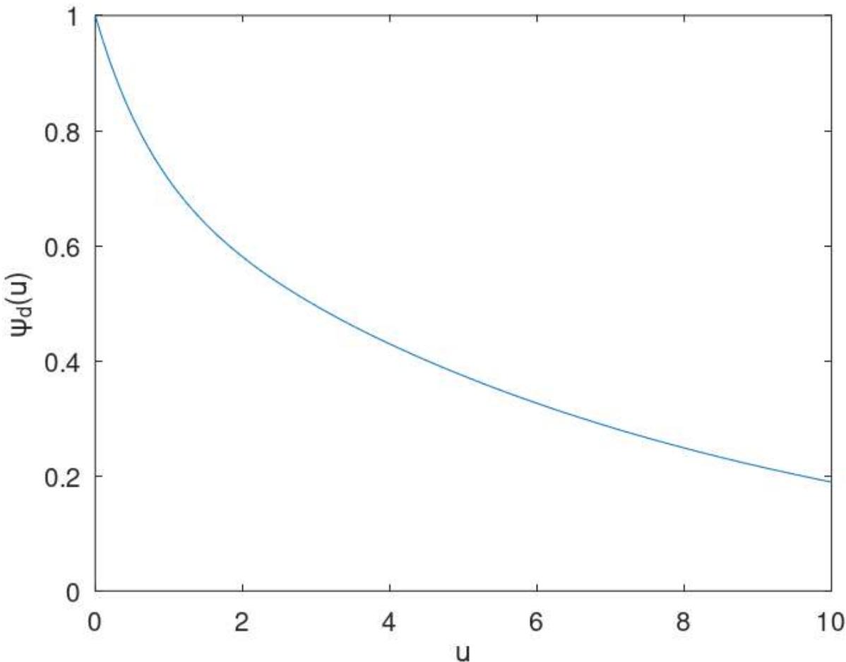
Example 2:
By setting the parameters ; and using using MATLAB, we present the curves associated with the probabilities due to oscillations.
In figures 1 and 2 illustrating the ruin probabilities caused by claims and by oscillations of the risk model, we notice that the ruin probabilities (caused by claims and by oscillations) both decrease as the initial capital increases.
{"image_source":{"path":"images/109496e2193623e2035c8f91379232e87e5279b1a70abfab95498e9eff9b9f16.jpg"},"content":"","chart_caption":[{"type":"text","content":"Figure 2: Ruin probability due to oscillations"}],"chart_footnote":[]}
Remark
IV. CONCLUSION
In this paper, we have determined the transforms of the insurer's loss probabilities and the ruin probabilities in a risk model with dependence perturbed by Brownian motion. To do this, we modelled the dependency structure between claim amounts and inter-claim times using the Spearman copula. The integral-differential equations and the Laplace transforms of the Gerber Shiu functions and the probabilities of ruin have been deduced by assuming that the losses are Erlang (2). In addition, some explicit expressions are obtained and numerical examples for the ruin probabilities for individual claim sizes with exponential distributions. This study can be made more practical by analysing dependency in a framework where policyholders are placed in two groups based on a threshold. This will be the subject of our next article.
5 Conflicts of Interest