A Paper on the Quantum-Mechanics of De-Sitter Space and the Aspects of Holography

Dr. Najmuj Sahadat Sarkar

IntelliPaper

− Abstract

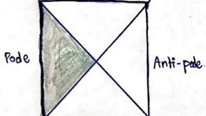
The main idea I want to discuss is the possibility that quantum-mechanical de Sitter space admits a holographic description. In spirit, such a description would be a boundary-like quantum system that makes no explicit reference to gravity, yet somehow encodes the physics of the bulk. Why focus on de Sitter space? Because de Sitter space is the “elephant in the room”: enormously large, highly symmetric, cosmologically relevant, and almost certainly closely related to the universe we inhabit. But unlike Anti–de Sitter space, de Sitter space has no natural boundary, which makes holography in this setting significantly more challenging. Despite this difficulty, researchers have explored many different perspectives. Discussions about de Sitter holography often resemble the story of the “Blind Men and the Elephant,” where each observer touches a different part and reaches a different conclusion. Some approaches emphasize dS/CFT, others TT̄ deformations, the swampland program, dS/dS duality, or matrix-theory–like constructions. None of these perspectives is clearly wrong, but none gives a complete picture. In this paper I present a set of “fragmentary circumstantial evidence’’ suggesting that certain aspects of de Sitter space may be described by a type of matrix theory. This idea was originally proposed by several theorists; here I revisit their arguments and add some additional clues.The framework I adopt is static-patch holography. A static patch is the region seen by an observer located at its center, which I call the “pode.” By symmetry, there is another static patch on the opposite side of the space, whose center I call the “anti-pode.” At time t = 0, spatial slices of de Sitter space resemble a sphere, with the pode at one end, the anti-pode at the other, and the cosmological horizon in the middle. At other times, one can naturally identify two horizons—one from each static patch. The basic hypothesis is that all physics inside a single static patch can be described by a holographic theory that is essentially quantum mechanics without gravity. De Sitter space behaves as a thermal system with temperature proportional to the inverse of the de Sitter radius, meaning larger de Sitter spaces are colder.The horizon carries an entropy proportional to its area. Defining this thermodynamics already assumes that the static patch is described by a unitary quantum system with a Hilbert

Made with Xodo PDF Reader and Editor Made with Xodo PDF Reader and Editor space, a Hamiltonian, and a set of symmetry generators that form the algebra of de Sitter space. In AdS, holographic degrees of freedom live at the asymptotic boundary. De Sitter space has no such boundary, and the static patch itself has none either. One might try to place the holographic degrees of freedom near the pode or anti-pode, but this fails because a small surface near the pode does not have enough area to encode the entire static patch. The only viable location is the stretched horizon. Therefore the holographic degrees of freedom must correspond to disturbances of the horizon itself. Operators that create excitations near the pode are complicated from the holographic viewpoint, while simple operators correspond to local changes of the horizon. This parallels what happens in AdS: excitations far from the holographic degrees of freedom appear as complex operators.In a thermal de Sitter background, rare Boltzmann fluctuations can move enough degrees of freedom from the horizon to the region near the pode, assembling macroscopic objects such as black holes. Such a configuration can be described by the Schwarzschild–de Sitter geometry, which contains two horizons: a small black hole horizon and a larger cosmological horizon. For sufficiently small black holes, the spacetime contains two identical black holes—one near the pode and one near the anti-pode. The spatial slice at t = 0 is a sphere with two small black hole horizons near the poles and the cosmological horizon at the equator. Assuming this configuration arises as a fluctuation, its probability is determined by the difference between the entropy of pure de Sitter space and the entropy of the configuration containing the black holes. The probability is exponentially suppressed, behaving like the exponential of minus the entropy difference. For small black holes, this entropy difference is proportional to the product of the de Sitter radius and the black hole mass, making such fluctuations extremely rare. This behavior is precisely what one expects from a finite quantum system with a horizon, and it strengthens the idea that the holographic description of the static patch may resemble a matrix-theory-type construction.

− Explore Digital Article Text

I. INTRODUCTION/CALCULATION

The primary aspect of quantum mechanical de Sitter space that I am talking about there is a holographic theory of the de Sitter space. In original sense, some kind of boundary theory based on conventional quantum mechanics which itself makes no explicit reference of gravity but which encodes the bulk the rest of space within the boundary, in a mysterious way which is not fully understandable But the question we ask, why we work with de Sitter space? I think, de Sitter space is the big elephant in the room! It's a elephant, because it's big! But de Sitter space is not only big but symmetrically big! And also it's important! We may have lived very similar to the de Sitter space! sometimes, we don't see the elephant in the room; perhaps it's just too big. But also sometimes, just because of our fear we pretended the elephant is not there. I think it's a good reason. But the main reason at least from the point of view of peoples, who doing certain kind of physics, last 15 or 20 years, we call it holographic physics. So the main reason is that de Sitter space has no boundary. It has not any natural boundary to anchor the holographic degrees of freedom to the boundary. So that makes the de Sitter space little bit of complicated. That does not mean that no body does not thinking about de Sitter space! When we thinking all the things and read about de Sitter space, another elephant analogy come to our mind. "The Elephant And The Blind Man" -analogy! Five blind man come close to the elephant and touch its different body parts. Just try to guessing what actually it is! And they all guessing wrong. Someone touch it's tail and say it's a rope! Someone touch its pointy horns or teeth and think it's a sword! But de Sitter conjecture with me or with my physics friend, like that it's dS/cFT, or its dS/dS, it's a swampland, or its just dS/dS, or probably just a Matrix‑theory! See, I don't say any of this is just wrong! But I have the feeling that, if we want to say the big picture, we would use different words! So what I am going to present today: Some "admittedly fragmentary circumstantial evidence", that de Sitter space or some aspects of the de Sitter space is described by a kind of matrix-theory. The kind of matrix-theory I'm talking about according to my knowledge: "first proposed by a group of theorists"! They proposed some "fragmentary circumstantial evidence", and I will show some more of it in this paper. And then come up on some other aspects of the de Sitter space! It's began to the idea of "Static Patch"! So the whole frame work, that I am going to discussing is the "Static Patch Holography" or "SPH"! The Static patch of the de Sitter space is the portion we seen from an observer at the center of that Static patch. I would like to call the center of that static patch "the Pole", and this static patch come-up with pair's, at the opposite end of the Static patch called "Anti-Pole"! So I called to Static patches, and pick one which is sort of "gauges choice", and then there is a natural opposing static patch on the other side of de Sitter space which I named "Anti-Pole"! And if we take a mid slice at the de Sitter space, that what you see at the left side a penrose diagram of de Sitter space. But on the right hand side there is an embedding diagram, through at time $t = 0$ , and What you can see is a metric sphere! The pole at one end, the anti‑pole at other end. And the horizon right middle here (fig:a)! If you don't want to slice it at $t = 0$ ; but some later time or before time then you have naturally two horizons! One associated with left static patch, and one associated with right static patch! So I draw them slightly separated (fig: a)! So the basic hypothesis is that all the physics inside of the Static patch can be described by the "Holographic theory". Again the holographic theory, mean the quantum mechanics especially the different version of quantum mechanics, which does not contain gravity! Here is the metric of the de-sitter space:

$\mathrm {f (r) = (1 - r ^ {2} / R ^ {2})}$ In this paper, I consider all the physics in 4d; not any higher number of dimension. r: the radial coordinate of a black hole! And R: is the radius of the de-sitter space. De-sitter space has thermodynamics! And it's natural the thermodynamics of the Static patch has a temperature T, which is equal to $1 / 2\pi \mathrm{R}$ . The bigger the space the colder it is! And it has some entropy which i called $\mathbf{S}_0$ : it's the starting basic entropy of the de-sitter space it-self! No perturbation in de-sitter space, just the static de-sitter space! And:

R² is the area of the horizon. But here are some hidden assumptions! In order to define the entropy or the temperature we make a huge assumption! Entropy is the part of statistical mechanics, basically quantum statistics! And to defining it we assume to make some assumptions. First of all unitary "quantum mechanics"! There are another kind of entropy that we usually don't use in general! So unitary quantum mechanics, in our case is the static patch! Or equivalently says, "A Hilbert Space Of States". It's possible to count the number of states! There is a Hamiltonian and a notion of energy! And important to distinguishing whether we really have the de-sitter space or rather than some other object! If we do quantum mechanics and look at the space, may be it describe a black hole, may be it describe something else! And i think, the important thing is the Symmetry of the de-sitter space! But in this paper, i don't want to describe about the Symmetry of de-sitter space! But it's very important the hamiltonian and the other generators of symmetry are that they close in a algebra $\mathrm{O}(4,1)$ : which is the Symmetry of de-sitter space! Let's now ask: where the holographic degrees of freedom resides! In the context of AdS they reside at the boundary of AdS! I mean the asymptotic cold boundary of "Anti de-sitter space" (AdS)! But de-sitter space has no boundary! The Static patch does not have any boundary! you most likely know that "the boundary of the static patch is it's horizon"! In the Penrose diagram of de-sitter space you might think the degrees of freedom reside at the boundary of pole and anti-pole! But that's doesn't work very well! Because it has a connection with covariant entropy bound! Means, that the region around the pole, if i draw a surface around the pole here (very close to the pole), then it's area will be very small! So the number of degress of freedom is sufficient to describe what inside the pole! But not the rest of the Static patch! So if you consider the entire static patch (fig: b), then the degrees of freedom or dof reside at horizon or symmetric horizon of de-sitter space! Now let me come to another question very briefly! I want to presume that the holographic degrees of freedom are some Q-bits, or they might be Matrix degrees of freedom, but I'm going to assume they are more simpler than that! So what are the simple degrees of freedom? If the holographic degrees of freedom reside at the stretched horizon, they have nothing to do any boundary, they don't have to do directly degrees of freedom near the pole! They have to do degrees of freedom or dof near the horizon! So thats not like to be the quasi normal modes! I mean the quasi normal modes of oscillation of the horizon! And also not the operators, which create simple disturbances near the pole! In AdS things are far from the holographic dof where they located! Those thing's tends to be complex! But things that are near the dof tends to be simple! So I would expect the dof associated with throwing something in from the pole, or the center of de-sitter space are corresponds to complex operators, and the simple operators have more to do with the disturbances of the horizon itself (fig:c)! So now I'm gonna do in this paper: "The Evidence That The Dof Of Holographic Description For De-sitter Matrix Theory!" The dof (degrees of freedom) or Holographic dof of particular kind! Means a particular way to describing What's in space??? So now, what we gonna talk about the boltzmann-fluctuation! Boltzmann fluctuations in thermal equilibrium are large scale fluctuations, crazy things, have normal frequency fluctuations, for example all the gases in the room, suddenly accumulated in one corner! So they are very very improbable! Here is an example: suppose we consider a de-sitter space, there are some degrees of freedom near the horizon! But then a crazy fluctuation happen and all the degrees of freedom near the horizon move and replace near the pole and anti-pole (fig: d)! There are enough degrees of freedom, so that they can form a macroscopic object! That is extremely improbable in the thermal equilibrium of de-sitter space! Imagine our de-sitter space will have in thermal equilibrium long long in future! But then a fluctuation occurs and a macroscopic object form near the pole and anti-pole! This is highly improbable, but this is possible, as any thing can possible in our de-sitter approximation, in thermal equilibrium! So the only question is what is the probability? So, let's talk about such fluctuations in little bit technical! Firstly take the fluctuations, so that they can form macroscopic object such as black hole, near the pole! The "de Sitter Schwarzschild metric" looks same as de-sitter metric, except that for black hole, there is a extra-term! "De-sitter Schwarzschild Metric" is given by:

f (r) = 1 - (r^{2} / R^{2}) - (2 M G / r) S o, n o w i f w e d o c r e a t e a b l a c k h o l e n e a r t h e p o l e, t h e r e w i l l b e t w o h o r i z o n s! I f w e s o l v e t h a t e q u a t i o n : O n e i s c o s m i c h o r i z o n, a n d t h e o t h e r h o r i z o n w i l l b e t h e h o r i z o n o f b l a c k h o l e! F r o m $ f (r) = 0 $, w e f i n d t h a t t h e r e a r e t w o p o s i t i v e s o l u t i o n s, a n d o n e n e g a t i v e w h i c h i s u n p h y s i c a l! W e c o m e u p o n t h i s t h i n g l a t e r! S o l e t^{'} s c o n c e n t r a t e o n s m a l l b l a c k h o l e s (f i g : e)! S m a l l b l a c k h o l e s a r e t h e b l a c k h o l e s, w h i c h a r e m u c h s m a l l e r t h a n t h e d e - s i t t e r r a d i u s, o r e q u i v a l e n t l y w h i c h e n t r o p y m u c h s m a l l e r t h a n t h e d e - s i t t e r e n t r o p y! H e r e i s t h e p e n r o s e d i a g r a m o f d e - s i t t e r S c h w a r z s c h i l d r a d i u s (f i g : e)! T h e r e a r e t w o h o r i z o n s; $ (r_{+}) $ t h e l a r g e r h o r i z o n, t h a t^{'} s t h e c o s m i c h o r i z o n! B e h i n d t h e $ r_{+} $ t h e s p a c e i s e x p o n e n t i a l l y e x p a n d! T h e o t h e r h o r i z o n i s t h e b l a c k h o l e h o r i z o n $ (r_{-}) $, w h i c h c o l l a p s e s t o t h e s i n g u l a r i t y, a n d t h e s p a c e i s p e r i o d i c! S o t h a t y o u c a n i d e n t i f y t h e l e f t d o t t e d l i n e w i t h t h e r i g h t d o t t e d l i n e! I t^{'} s a c t u a l l y t w o b l a c k h o l e; o n e i s o n p o l e s i d e a n d a n o t h e r o n e i s o n A n t i - p o l e s i d e! A n d t h e s p a t i a l g e o m e t r y a t $ t = 0 $, w h a t i t w o u l d l o o k l i k e ? ? ? H e r e i s t h e (f i g : f) g l o b a l s p h e r e! A t t h e m i d d l e, h e r e i s t h e c o s m i c r + h o r i z o n! B u t n e a r t h e p o l e a n d A n t i - p o l e t h e r e i s a s e c o n d h o r i z o n! T h e p o l e s i d e h o r i z o n i s s a m e a s t h e h o r i z o n a t A n t i - p o l e s i d e! S o, i t^{'} s p e r i o d i c i n n a t u r e! S o, t h a t^{'} s t h e g e o m e t r y o f S c h w a r z s c h i l d d e - s i t t e r (f i g : f)! N o w i w a n t t o t h i n k t h e S c h w a r z s c h i l d d e - s i t t e r i s j u s t a r e s u l t o f a f l u c t u a t i o n w h i c h c a n h a p p e n p r i m a r y d e - s i t t e r s p a c e! A n d w h a t i s t h e p r o b a b i l i t y f o r ? ? ? T h e p r o b a b i l i t y f o r i t :

\begin{array}{l} $\mathrm {P}$ = e^{-\Delta S} \ \Delta $\mathrm {S}$ = $\mathrm {S}$ _ {0} - $\mathrm {S}$ \ \end{array}

\Delta S = (\pi / G) \times \left[ R ^ {2} - \left(r ^ {2} _ {+} + r ^ {2} _ {-}\right) \right] $$ $\mathbf{r}^{2-}$ : That's the entropy associated with the cosmic horizon, and $\mathbf{r}^{2+}$ : is the entropy associated with the black hole! So the difference $\mathrm{S}_0 - \mathrm{S}$ is exactly the expression: $\Delta \mathrm{S}$ . If there is no black hole, then $\mathbf{r}_{+}$ is just capital "R"! And the entropy difference would be $\Delta S = 0$ ! And then the probability is just 1, but logically there would be no probability such as 1 or close to 1! Now, if you plug-in, what the value of $\mathbf{r}_{+}$ and $\mathbf{r}_{-}$ you get $\Delta S = 2\pi R M!$ You know it's not hard to do; and very straight forward! R: The size of de-sitter space, and M: is the mass of the black hole! So:

Δ S = 2 π R M $ 2 π RM $ : T h i s q u a n t i t y h e r e a l s o h a p p e n s t o b e b o l t z m a n n w e i g h t f o r t h e p r o d u c t i o n o f b l a c k h o l e! A n d $ 2 π R \sim 1 / T $ (o n e o v e r t h e t e m p e r a t u r e)! O r, $ 2 π R = β = T^{- 1} $; M i s a l s o t h e e n e r g y o f t h e b l a c k h o l e; $ 2 π R $ : i s t h e b o l t z m a n n w e i g h t a n d i t g o e s t o t h e e x p o n e n t a n d g i v e s y o u t h e p r o b a b i l i t y f o r s u c h a f l u c t u a t i o n t o b e h a p p e n! T h e r e i s a n o t h e r f o r m w h i c h i f i n d v e r y i n t e r e s t i n g! I t h a s h i g h e r d i m e n s i o n a l g e n e r a l i z a t i o n! B i g " R " i s t h e s q u a r e r o o t o f e n t r o p y i n d e - s i t t e r s p a c e! B i g " M " i s p r o p o r t i o n a l t o t h e e n t r o p y o f b l a c k h o l e! S o i f y o u p u t t h i s t o g e t h e r a n d g o t h r o u g h t h e c a l c u l a t i o n y o u m a y f i n d : $ $ Δ S = \sqrt{S_{0} \cdot s} $ $ K e e p t h i s f o r m u l a i n m i n d, b e c a u s e t h e r e i s a h i n t (o r, a c l u e) a b o u t t h e s t r u c t u r e o f d e g r e e s o f f r e e d o m! T h a t c l u e f i r s t d i s c u s s e d i n 2006, a n d l a t e r b y L . S u s s k i n d (2011)! S o t h e c l u e o r t h e r e s u l t o f t h e c l u e i n s i d e t h e m a t r i x - t h e o r y! I m e a n, t h e m a t r i x s t r u c t u r e f o r t h e d e g r e e s o f f r e e d o m i n d e - s i t t e r s p a c e (f i g : g)! L e t^{'} s s t a r t w i t h m a t r i x w i t h b i g s q u a r e a r r a y s, $ N \times N $ o f t h e m (f i g : g)! R o u g h l y s p e a k i n g m a t r i c e s s h o w - u p i n t h e t h e o r y o f " D ‑ b r a n e "! Y o u c a n t h i n k o f t h i s D ‑ b r a n e; b u t I t h i n k y o u d o n^{'} t h a v e t o! T h e d i a g o n a l e l e m e n t s r e p r e s e n t t h e p o s i t i o n o f D ‑ b r a n e! B u t f o r t h e m o m e n t t h e y a r e m a t r i c e s, a n d I^{'} m g o i n g t o a s s u m e i n t h e r m a l e q u i l i b r i u m; a l l o f t h i s m a t r i x e l e m e n t s a r e t h e d e g r e e s o f f r e e d o m! S o t h e r e a r e $ N^{2} = $ d e g r e e s o f f r e e d o m! A n d i n t h e r m a l e q u i l i b r i u m e a c h o f o n e c a r r y s o m e e n t r o p y! A n d t h e t o t a l e n t r o p y i s p r o p o r t i o n a l t o t h e n u m b e r o f D e g r e e s o f f r e e d o m! M e a n s, $ S_{0} = σ N^{2} $ : r e p r e s e n t e n t r o p y p e r l i t t l e d e g r e e o f f r e e d o m! I f y o u a s k m e H o w y o u c a l c u l a t e ? A c t u a l l y i d o n^{'} t k n o w, h o w t o c a l c u l a t e! S o j u s t c a l l e d i t 0! N o w h o w c a n w e d e s c r i b e a s y s t e m i n m a t r i x t h e o r y ? I a m c o m i n g - u p o n t h e o r i g i n a l " B F S S " - m a t r i x t h e o r y (f i g : h)! B u t i n t h i s p a p e r i d o n^{'} t d e s c r i b e t h e " B F S S " - m a t r i x t h e o r y m o r e d e t a i l, i t^{'} s j u s t a n i n s p i r a t i o n a s y o u m i g h t t h i n k! H o w w e w o u l d t h i n k a b o u t s o m e s y s t e m w h i c h d i v i d e d i n t o t w o s u b s y s t e m! I n t h i s c a s e, t h e t w o d i v i d e d s u b - s y s t e m a r e t h e " H o r i z o n d e g r e e s o f f r e e d o m ", a n d " T h e h o r i z o n t h a t s e p a r a t e d t h e t w o b l a c k h o l e s " (s e e f i g : h)! O n e w h o s t u d i e d m a t r i x t h e o r y g i v e y o u a q u i c k a n s w e r! O n e b l o c k o f t h e m a t r i x a s s o c i a t e d w i t h o n e - d e g r e e s o f f r e e d o m, a n d t h e o t h e r b l o c k a s s o c i a t e d w i t h t h e o t h e r d e g r e e s o f f r e e d o m! T h e o f f - d i a g o n a l e l e m e n t s a r e u n e x c i t e d! C l a s s i c a l l y S a y^{'} s, t h i s o f f - d i a g o n a l m a t r i x e l e m e n t s a r e s e t t o b e z e r o! T h e s m a l l s u b s y s t e m i n " B F S S " - m a t r i x h a v e $ m \times m $ d e g r e e s o f f r e e d o m, a n d t h e b i g s u b s y s t e m i n " B F S S " - m a t r i x h a v e $ (N - m)^{2} $ d e g r e e s o f f r e e d o m! S o : $ S = σ \cdot (N - m)^{2} $ : C o s m i c H o r i z o n E n t r o p y! S = σ m^{2} : B l a c k H o l e H o r i z o n E n t r o p y! A f t e r t h e r m a l f l u c t u a t i o n s, t h e e n t r o p y o f c o s m i c h o r i z o n d e c r e a s e s, t h a t m e a n s t h e r e a r e f e w d e g r e e s o f f r e e d o m i n t h e r m a l e q u i l i b r i u m! S o, t h e c o n d i t i o n e n t r o p y $ S < S_{0}! $ i s t h e o r i g i n a l e n t r o p y i n d e - s i t t e r s p a c e! A n d t h e b l a c k h o l e e n t r o p y $ s = σ \cdot m^{2} $ S o, n o w w h a t a b o u t $ Δ S ? ? ? $

\Delta S = S_0 - S - s

\Delta $\mathrm {S}$ = \sigma \cdot $\mathrm {N}$ ^ {2} - \sigma \cdot ( $\mathrm {N}$ - $\mathrm {m}$ ) ^ {2} - \sigma \cdot $\mathrm {m}$ ^ {2}

\Delta $\mathrm {S}$ = 2 \sigma ( $\mathrm {m}$ \cdot $\mathrm {N}$ )

$ Δ S $ : i s s i m p l y t h e n u m b e r o f c o n s t r a i n t s $ \times σ $! I f w e l o o k e d a t t h e " B F S S " - m a t r i x s t r u c t u r e; w e m a y f i n d o u t t h a t (f i g : h) t h e r e a r e t w o o f f - d i a g o n a l m a t r i x s t r u c t u r e s, w h e r e o f f - d i a g o n a l e l e m e n t s a r e s e t t o z e r o! S o t h a t t h e e n t r o p y d i f f e r e n c e b y c o n s t r a i n i n g t h e s y s t e m i n t h a t w a y! $ $ Δ S = 2 \sqrt{S \times s} $ $ T h e b i g " S " p r o p o r t i o n a l t o $ \sim (N - m)^{2} $ o r $ (N - m) \sim \sqrt{S}) $ A n d s m a l l " s " i s p r o p o r t i o n a l t o $ \sim m^{2} $, o r $ m \sim \sqrt{s}! $ A n d t h e w h o l e r e s u l t i s $ 2 \sqrt{(S ∙ s)} $ . $ Δ S = 2 \sqrt{(S ∙ s)} $ i s e x a c t l y t h e s a m e f o r m u l a t h a t i d e r i v e d - o u t s t a r t i n g w i t h t h e d e - s i t t e r S c h w a r z s c h i l d b l a c k h o l e! A n d c a l c u l a t i n g t h e e n t r o p y d i f f e r e n c e! I t^{'} s l i l, b i t o f s u r p r i s e t h a t t h e y t w o m a t c h t o g e t h e r d e s p i t e t h e f a c t o r o f 2! T h e e n t r o p y i s t h e p r o d u c t o f t w o s u b s y s t e m e n t r o p y i s n o t a n o r m a l t h i n g! I t^{'} s n o t t h e t h i n g t h a t w e s e e e v e r y d a y! B e c a u s e t h e g e n e r a l r e l a t i v i s t i c c a l c u l a t i o n o f $ Δ S $, a n d M a t r i x c a l c u l a t i o n o f $ Δ S $ i s j u s t e q u a l t o e a c h o t h e r! L e t m e g i v e a n e x a m p l e w h i c h d o e s n o t g i v e t h a t t y p e o f f o r m u l a! H e r e i s t h e " T o y - M o d e l " (s e e f i g : i)! (f i g : i) Y o u h a v e a p o t e n t i a l w h i c h h a s a " p e a k " a t t h e c e n t e r, a " u p s i d e d o w n " h a r m o n i c o s c i l l a t o r, a n d a l l o f t h e p a r t i c l e s o r m o s t o f t h e p a r t i c l e s s i t a t t h e b o t t o m o f (m i n i m u m) t h e p o t e n t i a l! A n d g i v e t h e s y s t e m a l a r g e e n t r o p y! I n t h e r m a l e q u i l i b r i u m t h e p a r t i c l e s t y p i c a l l y s i t a t t h e b o t t o m o f t h e w e l l! B u t t h e r e i s a t i n y p r o b a b i l i t y t h a t t h e p a r t i c l e s o r s o m e p a r t i c l e s i t t o p o f t h e p o t e n t i a l, d u e t o t h e r m a l f l u c t u a t i o n s! I w o n^{'} t g o t h r o u g h t h e c a l c u l a t i o n s, i t^{'} s e l e m e n t a r y j u s t e l e m e n t a r y s t a t i s t i c a l m e c h a n i c s! $ $ Δ S = m \cdot \log (\frac{V}{v}) = 2 m \cdot \log (\frac{s}{S_{0}}) $ $ Δ S \sim m \cdot \log (m / N) Δ S \sim s \cdot \log (s / S)

So, the $\Delta S$ or differential entropy, proportional to the entropy of small subsystem (where few degrees are sit on) times logarithm of small subsystem entropy "s": $-$ : logarithm of large subsystem entropy "S"! And it does not like anything like the product: \Delta S = 2 \sigma N \cdot m \sim $\sqrt {(s \cdot S)}$

There are many of the mode you can construct and none of them looked like  $\sim \sqrt{(\mathrm{s} \cdot \mathrm{S})} \rightarrow$  this! Except the matrix construction! So this type of formula  $\Delta \mathrm{S} \sim \sqrt{(\mathrm{s} \cdot \mathrm{S})}$  intimately connected with the constraints  $\Delta \mathrm{S}$  formula connected with little "m" and "(N-m) So,  $\Delta \mathrm{S} \approx \sqrt{(\mathrm{s} \cdot \mathrm{S})}$  show's a very interesting correspondence between "Matrix-theory"; "Statistical Mechanics"; and "Schwarzschild de Sitter!! Now i come-up on a very difficult problem; not too much difficult! But giving up the assumptions, of small black holes, we study various kind of black holes of entire mass range; from smaller possible black holes, to large mass black holes in de Sitter space!.

# II. FOR LARGE BLACK HOLES

( $\mathrm {s}$ / $\mathrm {S}$ ) {\sim} 1

\mathrm {f (r) = 1 - (r ^ {2} / R ^ {2}) - (2 M G / r)}

\mathrm {f(r) = r - (r ^ {3} / R ^ {2}) - 2 M G = 0}

$\operatorname {f}$ ( $\mathrm {r}$ ) = 0

$\mathrm {X}$ = \left[ ( $\mathrm {r}$ _ {-}) - ( $\mathrm {r}$ _ {+}) \right] / $\mathrm {R}$

1 < X < 1

\Delta S = \Delta S _ {n} \cdot [ 1 - X ^ {2} ]

\Delta $\mathrm {S}$ = \Delta $\mathrm {S}$ _ { $\mathrm {n}$ }

A n d i f y o u c a l c u l a t e t h e e n t r o p y d i f f e r e n c e a t N, B e f o r e t u r n i n g i n t o t h e m a t r i x t h e o r y, l e t s i m a g i n e a t r a n s i t i o n! T h e t r a n s i t i o n s t a r t s a t $ X = - 1 $ . T h a t^{'} s m e a n t h e T i n y - T i n y b l a c k h o l e i n t h e b i g d e - s i t t e r s p a c e! N o w l e t^{'} s i m a g i n e t h e T i n y - T i n y b l a c k h o l e s t a r t s a b s o r b i n g e n e r g y f r o m t h e c o s m i c h o r i z o n! N o w, y o u m i g h t b e s a y t h a t v i o l a t e t h e 2 n d l a w o f T h e r m o d y n a m i c s! y o u g e t $ Δ S = (1 / 3) ∙ S_{n} $! H e r e $ (1 / 3) $ j u s t a n u m e r i c a l c o n s t a n t! $ S_{0} $ i s t h e e n t r o p y o f d e - s i t t e r s p a c e a t t h e r m a l e q u i l i b r i u m! T h a t^{'} s c a l c u l a t i o n i s v e r y e a s y t o d o, a s t h e r e i s a l o t o f s y m m e t r y! B u t i f y o u g o f a r f r o m t h e S y m m e t r y p o i n t t h e a n s w e r b e c o m e s v e r y h a r d t o d e f i n i n g! B u t i t^{'} s n o t h a r d a t t h e p o i n t N . I f $ X = 0 $, t h e n a c c o r d i n g t o t h e f o r m u l a b l a c k h o l e s h r i n k s i n t o z e r o s i z e, a n d h e n c e t h e r e i s n o $ Δ S $! J u s t : O u r h o r i z o n i s m u c h c o l d e r t h a n t h e b l a c k h o l e! S o i t v i o l a t e t h e 2 n d l a w o f t h e r m o d y n a m i c s! B u t t h e 2 n d l a w o f t h e r m o d y n a m i c s n o t a l a w! I t^{'} s j u s t a s t a t i s t i c a l t e n d e n c y! I t^{'} s s i m p l y i m p r o b a b l e f o r e n e r g y t o f l o w f r o m t h e c o s m i c h o r i z o n t o b l a c k h o l e h o r i z o n! S o, d o n^{'} t w o r r y a b o u t! I w i l l s h o w y o u i n a m o m e n t!!! B u t l e t^{'} s t a k e t h a t t h e r e i s a b o l t z m a n n f l u c t u a t i o n, s o e n e r g y c a n f l o w f r o m c o s m i c h o r i z o n t o b l a c k h o l e! A n d i n t h a t c a s e t h e b l a c k h o l e b e g i n t o g r o w! E v e n t u a l l y t h e b l a c k h o l e h o r i z o n a n d t h e c o s m i c h o r i z o n i n s a m e s i z e a t t h e p o i n t " N "! B u t i f i t k e e p s g o i n g, t h e n c o s m i c h o r i z o n s h r u n k b a c k a n d b e c o m e B l a c k H o l e H o r i z o n! O r m a y b e n o b l a c k h o l e a t a l l . S o, N o w w e f i n d B l a c k h o l e h o r i z o n b e c o m e t h e c o s m i c h o r i z o n! I w i l l c a l l i t " I n s i d e - O u t " t r a n s i t i o n (S e e t h e f i g : l) * . S o f o r a n o b s e r v e r (s e e f i g : m) * f i r s t t h e t i n y b l a c k h o l e a b s o r b e n e r g y f r o m d e - s i t t e r s p a c e a n d g r o w! A t s o m e p o i n t o r " N " p o i n t t h e b o t h c o s m i c a n d b l a c k h o l e h o r i z o n a t s a m e s i z e! A n d t h e n t h e b l a c k h o l e h o r i z o n g r o w a n d b e c o m e t h e c o s m i c h o r i z o n a n d t h e c o s m i c h o r i z o n t u r n i n t o a t i n y - b l a c k h o l e h o r i z o n h o l e h o r i z o n! A n d t h e p r o b a b i l i t y f o r t h i s t o h a p p e n :

\begin{array}{l} P_{ $\text{prob}$ } = e^{-\Delta S} = e^{-\left(S_{0}/3\right)} \ \end{array}

\Delta S = \sigma m \cdot (N - m)

\begin{array}{l} $\mathrm {S}$ \sim $\mathrm {r}$ ^ {2} \ $\text {And}$ ( $\mathrm {r}$ _ {-}) = \sqrt {\mathrm {S} _ {-}}; ( $\mathrm {r}$ _ {+}) = \sqrt {\mathrm {S} _ {+}} \ \mathrm {So: X = [ (r _ {-}) - (r _ {+}) ] / R} \ = [ (\sqrt {S _ {-}}) - (\sqrt {S _ {+}}) ] / \sqrt {S _ {0}} \ = [ $\mathrm {m}$ - ( $\mathrm {N}$ - $\mathrm {m}$ ) ] / $\mathrm {N}$ \ = (2 $\mathrm {m}$ / $\mathrm {N}$ ) - 1 \ \end{array}

\Delta S = \Delta S _ {n} \cdot [ 1 - X ^ {2} ]

\Delta $\mathrm {S}$ _ { $\mathrm {n}$ } \sim ( $\mathrm {S}$ _ {0} / 2)

$\mathrm {L}$ = \sum $\mathrm {Tr}$ ( $\mathrm {c}$ ^ {2} $\mathrm {R}$ ^ {4} $\mathrm {A}$ ^ {2} - [ \Re , $\mathrm {A}$ ] [ $\mathrm {A}$ , \Re ]) + \dots \dots \dots .

$\mathrm {L}$ = $\mathrm {c}$ ^ {2} $\mathrm {R}$ ^ {4} $\mathrm {a}$ _ { $\mathrm {i j}$ } $\mathrm {a}$ _ { $\mathrm {j i}$ } - $\mathrm {R}$ ^ {2} $\mathrm {a}$ _ { $\mathrm {i j}$ } $\mathrm {a}$ _ { $\mathrm {j i}$ }

$a_{ij}a_{ji}$  are the quadratic terms in time derivative, and  $a_{ij}a_{ji}$  are quadratic terms in a's.


# III. CONCLUSION

So, what you get by this result that I finally derived? You get a system of harmonic oscillator. If you work out the frequency of the harmonic oscillator you may get:

\omega = 1 / $\mathrm{cR}$

$\mathrm{T}$ = 1 / 2 \pi $\mathrm{R}$

\Delta S = 2 \left(\sigma^ {\prime} / \sigma\right) \times $\sqrt {(s \cdot S)}$ \approx $\sqrt {(s \cdot S)}$

(\sigma^ {\prime} / \sigma) _ { $\text {small}$ } \approx 1 / 2

\Delta S = (1 / 2) \cdot (\sigma^ {\prime} / \sigma) S _ {0} (1 - X ^ {2})

\approx (1 / 3) \times S _ {0} \cdot (1 - X ^ {2})

(\sigma^ {\prime} / \sigma) _ {-} $\text {big}$ \approx 2 / 3

DOF = $\mathrm{Finite}$

A = \left[ \begin{array}{l l l l} a_{11} & a_{12} & a_{13} & \dots \ a_{21} & \cdot & \cdot & \cdot \ \vdots & \cdot & \cdot & \cdot \ \vdots & \cdot & \cdot & \cdot \ \vdots & \cdot & \cdot & \cdot \ \vdots & \cdot & \cdot & \cdot \ a_{n1} & & \cdot & \cdot \end{array} \right]; S _ {0} = \sqrt {N ^ {2}}

fig: (g)

$\mathbf {R}$ = \left[ \begin{array}{l l l l l} r_{11} & r_{12} & r_{13} & \dots & r_{1n} \ r_{21} & \bullet & & & \ \bullet & & \bullet & & \ \bullet & & \bullet & & \ \bullet & & & \bullet & \ r_{n1} & & & & \end{array} \right]

$\mathrm{fig}$ : (P)

R =

\begin{array}{r l} & {\left[ \begin{array}{l l l l l} R & 0 & 0 & 0 & 0 \ 0 & R & 0 & 0 & 0 \ 0 & 0 & R & 0 & 0 \ 0 & 0 & 0 & R & 0 \ 0 & 0 & 0 & 0 \end{array} \right],} \ & {\left[ \begin{array}{l l l l l} 0 & 0 & 0 & 0 & 0 \ 0 & 0 & 0 & 0 & 0 \end{array} \right]} \end{array}

$\mathrm{fig}$ : (g)

− Conflict of Interest

The authors declare no conflict of interest.

− Ethical Approval

Not applicable

− Data Availability

The datasets used in this study are openly available at [repository link] and the source code is available on GitHub at [GitHub link].

− Funding

This work did not receive any external funding.

− Cite this article

Generating citation...

Submission received 22 November 2025
Peer Review Double Blind Handling Editor
Accepted 28 November 2025 Access Review Comments
Online published 15 December 2025

Special Issue

Launch a focused special issue to highlight research, emerging trends, and expert insights in your academic field.

Classification
1

LCC Code: QB500.268, QC173.6, QC174.12
Version of record

v1.0
Issue date

15 December 2025
Language

en

A Paper on the Quantum-Mechanics of De-Sitter Space and the Aspects of Holography

Download Article Access OJS

Open Access

Research Article

CC-BY-NC 4.0

LJRS Volume 25 LJRS Volume 25 Issue 15, Pg. 25-44

Explore Journal

Read LJRS Volume 25 Issue 15 Explore LJRS Volume 25

A Paper on the Quantum-Mechanics of De-Sitter Space and the Aspects of Holography

IntelliPaper

− Abstract

− Explore Digital Article Text

I. INTRODUCTION/CALCULATION

− Conflict of Interest

− Ethical Approval

− Data Availability

− Funding

− Cite this article

− Related Research

Request Review Access

Order Article Reprints

Special Issue

Classification

Version of record

Issue date

Language

Privacy preferences