Analysis and Control of Malaria Dynamic Models

# I. BACKGROUND Romero-Leiton, et al. (2019)[1] conducted stability analysis and discussed optimal control intervention strategies of a malaria mathematical model. Ibrahim et al. (2020)[2] investigated the impact of awareness on controlling malaria disease using a mathematical modelling approach. Abioye Adesoye Idowu, et al. (2020)[3] performed optimal control on a mathematical model of malaria. Kobe (2020)[4], developed a mathematical model of controlling the Spread of Malaria Disease Using Intervention Strategies. Ndii et al. (2021)[5] studied the effects of individual awareness and vector controls on malaria transmission dynamics using multiple optimal control. Adepoju et al. (2021)[6] discussed the stability and optimal control of a disease model with vertical transmission and saturated incidence. Keno et al. (2021)[7] discussed optimal control and cost effectiveness analysis of SIRS malaria disease model with temperature variability factor. Aldila Dipo et al. (2021)[8] studied an optimal control problem and backward bifurcation on malaria transmission with vector bias. Tasman, et al. (2021)[9] researched an optimal control problem of a malaria model with seasonality effect using real data. Al Basir et al. (2021)[10] explored the effects of awareness and time delay in controlling malaria disease propagation. Sinan Muhammad et al. (2022)[11], developed a Fractional mathematical model of malaria disease with treatment & insecticides. Al Basir et al. (2023)[12] published an article on mathematical modelling and optimal control of malaria using awareness-based interventions. Olaniyi Samson et al. (2023)[13], performed an optimal control analysis of a mathematical model for recurrent malaria dynamics. Wako et al (2025)[14] analysed and performed optimal control calculations of a model describing malaria and its associated complications. This work aims to perform bifurcation analysis and multiobjective nonlinear control (MNLMPC) studies in two measles transmission models, which are discussed in Al Basir et al (2023) (model 1) [13] and Wako et al (2025) [14](model 2). The paper is organized as follows. First, the model equations are presented, followed by a discussion of the numerical techniques involving bifurcation analysis and multiobjective nonlinear model predictive control (MNLMPC). The results and discussion are then presented, followed by the conclusions. # II. MODEL EQUATIONS (MODEL 1) AL BASIR ET AL (2023) In model 1, hu, ha, and hi represent the susceptible unaware, susceptible, aware, and infected human populations. vs and vi represent the susceptible and infected vector populations, while mv represents the level of awareness. The model equations are $$ \frac {d(hu)}{d t} = \pi_h - \alpha hu (mv) - \frac {\lambda_1 (hu) vi}{nv} - d_h (hu) + \frac {g(ha)}{1 + mv} $$ $$ \frac {d(ha)}{d t} = \alpha hu (mv) - d_h (ha) + c_1 r (hi) mv - \frac {\lambda_2 (ha) vi}{nv} - \frac {g (ha)}{1 + mv} $$ $$ \frac {d (hi)}{d t} = \frac {\lambda_1 (hu) vi}{nv} - \left(d_h + \delta\right) hi - c_1 r (hi) mv + \frac {\lambda_2 (ha) vi}{nv} $$ $$ \frac {d (vs)}{d t} = \pi_v - \frac {\beta (hi) vs}{nv} - \mu vs - c_2 \gamma (vs) mv $$ $$ \frac {d (vi)}{d t} = \frac {\beta (hi) vs}{nv} - \mu vi - c_2 \gamma vi (mv) $$ $$ \frac {d (mv)}{d t} = c_3 \omega + \sigma hi - \theta mv $$ The base parameter values are $$ \lambda_1 = 0.02; \alpha = 0.001; \lambda = 0.002; \beta = 0.25; \pi_h = 400; \pi_v = 10000; $$ $$ \mu = 0.12; r = 0.001; d_h = 0.002; \delta = 0.01; \gamma = 0.003; \theta = 0.01; $$ $$ c_1 = 0.2; c_2 = 0.2; c_3 = 0.2; g = 0.01; \omega = 0.05; \sigma = 0.05; $$ c_1, c_2 and c_3 are the control parameters. More details can be found in Al Basir et al (2023). # III. MODEL EQUATIONS (MODEL 2) WAKO ET AL (2025) Model 2 is a scaled model where sh, im, ic, rh, are the scaled variables representing the susceptible humans, malaria-infected humans, those with induced complications, and recovered human beings. The scaled susceptible and infected mosquito populations are represented by sv and iv. The model equations are $$ g_{fac} = \frac {\gamma_1}{1 + \varepsilon i_c} $$ $$ \frac {d (s_h)}{d t} = \\mu_1 - \\alpha_1 \sigma q (i_v) s_h - \\mu_1 s_h $$ $$ \frac {d (i_m)}{d t} = \\alpha_1 \sigma q (i_v) s_h - (\\omega_1 + \\mu_1) i_m - \\gamma_0 (u_0) i_m $$ $$ \frac {d (i_c)}{d t} = \\omega_1 (i_m) - \\mu_1 (i_c) - u_1 (g_{fac}) i_c - \\delta_0 (i_c) $$ $$ \frac {d (r_h)}{d t} = \\gamma_0 (u_0) i_m + u_1 (g_{fac}) i_c - \mu_1 (r_h) $$ $$ \frac {d (s_v)}{d t} = \\mu_2 - \\alpha_2 \sigma (i_m) s_v - \\mu_2 (s_v) $$ $$ \frac {d (i_v)}{d t} = \\alpha_2 (\sigma) i_m (s_v) - \\mu_2 (i_v) $$ The base parameter values are $$ \alpha_1 = 0.75; \alpha_2 = 0.2; \sigma = 0.3; \mu_1 = 3.9139e-05; \\mu_2 = 0.12; \omega_1 = 0.2185; \\gamma_0 = 0.0056; $$ $$ \\gamma_1 = 0.0056; \delta_0 = 0.0244; \\varepsilon = 0.007; q = 2; u_0 = 0.2; u_1 = 0.2; $$ More details can be found in Wako et al (2025). # IV. BIFURCATION ANALYSIS The MATLAB software MATCONT is used to perform the bifurcation calculations. Bifurcation analysis deals with multiple steady-states and limit cycles. Multiple steady states occur because of the existence of branch and limit points. Hopf bifurcation points cause limit cycles. A commonly used MATLAB program that locates limit points, branch points, and Hopf bifurcation points is MATCONT (Dhooge Govaerts, and Kuznetsov, 2003[15]; Dhooge Govaerts, Kuznetsov, Mestrom and Riet, 2004[16]). This program detects Limit points(LP), branch points(BP), and Hopf bifurcation points(H) for an ODE system $$ \frac {d x}{d t} = f (x, \alpha) $$ $x \in R^n$ Let the bifurcation parameter be $\alpha$ . Since the gradient is orthogonal to the tangent vector, The tangent plane at any point $w = \left[w_{1},w_{2},w_{3},w_{4},\dots w_{n + 1}\right]$ must satisfy $$ A w = 0 $$ Where A is $$ A = \left[ \begin{array}{c c} \partial f / \partial x & | \partial f / \partial \alpha \end{array} \right] $$ where $\partial f / \partial x$ is the Jacobian matrix. For both limit and branch points, the Jacobian matrix $J = [\partial f / \partial x]$ must be singular. For a limit point, there is only one tangent at the point of singularity. At this singular point, there is a single non-zero vector, $\mathbf{y}$ , where $\mathrm{Jy} = 0$ . This vector is of dimension $n$ . Since there is only one tangent the vector $y = (y_{1},y_{2},y_{3},y_{4},\ldots y_{n})$ must align with $\hat{w} = (w_1,w_2,w_3,w_4,\dots w_n)$ . Since $$ J \hat {w} = A w = 0 $$ the $n + 1$ th component of the tangent vector $\mathcal{W}_{n + 1} = 0$ at a limit point (LP). For a branch point, there must exist two tangents at the singularity. Let the two tangents be $z$ and $w$ . This implies that $$ A z = 0 $$ $$ A w = 0 $$ Consider a vector $\mathbf{v}$ that is orthogonal to one of the tangents (say $\mathbf{w}$ ). $\mathbf{v}$ can be expressed as a linear combination of $\mathbf{z}$ and $\mathbf{w}$ ( $\nu = \alpha z + \beta w$ ). Since $A z = A w = 0$ ; $A v = 0$ and since $\mathbf{w}$ and $\mathbf{v}$ are orthogonal, $w^{T}v = 0$ . Hence $B\nu = \begin{bmatrix} A \\ w^{T} \end{bmatrix}\nu = 0$ which implies that B is singular. Hence, for a branch point (BP) the matrix $B = \begin{bmatrix} A \\ w^T \end{bmatrix}$ must be singular. At a Hopf bifurcation point, $$ \det \left(2 f _ {x} (x, \alpha) @ I _ {n}\right) = 0 $$ @ indicates the bialternate product while $I_{n}$ is the n-square identity matrix. Hopf bifurcations cause limit cycles and should be eliminated because limit cycles make optimization and control tasks very difficult. More details can be found in Kuznetsov (1998[17]; 2009[18]) and Govaerts [2000] [19]. # V. MULTIOBJECTIVE NONLINEAR MODEL PREDICTIVE CONTROL(MNLMPC) The rigorous multiobjective nonlinear model predictive control (MNLMPC) method developed by Flores Tlacuahuaz et al (2012)[20] was used. Consider a problem where the variables $\sum_{t_i = 0}^{t_i = t_f}q_j(t_i)$ (j=1, 2..n) have to be optimized simultaneously for a dynamic problem $$ \frac {d x}{d t} = F (x, u) $$ $t_{f}$ being the final time value, and n the total number of objective variables and u the control parameter. The single objective optimal control problem is solved individually optimizing each of the variables $\sum_{t_i = 0}^{t_i = t_f}q_j(t_i)$ The optimization of $\sum_{t_i = 0}^{t_i = t_f}q_j(t_i)$ will lead to the values $q_{j}^{*}$ . Then, the multiobjective optimal control (MOOC) problem that will be solved is $$ \min \left(\sum_{j=1}^{n} (\sum_{t_i=0}^{t_f} q_{j}(t_{i}) - q_{j}^{*})\right)^{2} $$ $$ subject to \quad \frac {d x}{d t} = F (x, u); $$ This will provide the values of u at various times. The first obtained control value of u is implemented and the rest are discarded. This procedure is repeated until the implemented and the first obtained control values are the same or if the Utopia point where $\left(\sum_{t_i = 0}^{t_i = t_f}q_j(t_i) = q_j^*\right)$ for all j) is obtained. Pyomo (Hart et al, 2017)[21] is used for these calculations. Here, the differential equations are converted to a Nonlinear Program (NLP) using the orthogonal collocation method. The NLP is solved using IPOPT (Wächter And Biegler, 2006)[22] and confirmed as a global solution with BARON (Tawarmalani, M. and N. V. Sahinidis 2005)[23]. The steps of the algorithm are as follows 1. Optimize $\sum_{t_i = 0}^{t_i = t_f}q_j(t_i)$ and obtain $q_{j}^{*}$ . 2. Minimize $\left(\sum_{j=1}^{n}\left(\sum_{t_{i}=0}^{t_{i}=t_{f}} q_{j}\left(t_{i}\right)-q_{j}^{*}\right)\right)^{2}$ and get the control values at various times. 3. Implement the first obtained control values 4. Repeat steps 1 to 3 until there is an insignificant difference between the implemented and the first obtained value of the control variables or if the Utopia point is achieved. The Utopia point is when $$ \sum_ {t _ {i = 0}} ^ {t _ {i} = t _ {f}} q _ {j} \left(t _ {i}\right) = q _ {j} ^ {*} \quad \text{for all j.} $$ Sridhar (2024)[24] demonstrated that when the bifurcation analysis revealed the presence of limit and branch points the MNLMPC calculations to converge to the Utopia solution. For this, the singularity condition, caused by the presence of the limit or branch points was imposed on the co-state equation (Upreti, 2013)[25]. If the minimization of $q_{1}$ leads to the value $q_{1}^{*}$ and the minimization of $q_{2}$ leads to the value $q_{2}^{*}$ , The MNLMPC calculations will minimize the function $(q_{1} - q_{1}^{*})^{2} + (q_{2} - q_{2}^{*})^{2}$ . The multiobjective optimal control problem is $\min_{\substack{(q_1 - q_1^*)^2 + (q_2 - q_2^*)^2 \\ }}$ subject to $\frac{dx}{dt} = F(x,u)$ Differentiating the objective function results in $$ \frac {d}{d x _ {i}} \left(\left(q _ {1} - q _ {1} ^ {*}\right) ^ {2} + \left(q _ {2} - q _ {2} ^ {*}\right) ^ {2}\right) = 2 \left(q _ {1} - q _ {1} ^ {*}\right) \frac {d}{d x _ {i}} \left(q _ {1} - q _ {1} ^ {*}\right) + 2 \left(q _ {2} - q _ {2} ^ {*}\right) \frac {d}{d x _ {i}} \left(q _ {2} - q _ {2} ^ {*}\right) $$ The Utopia point requires that both $(q_{1} - q_{1}^{*})$ and $(q_{2} - q_{2}^{*})$ are zero. Hence $$ \frac {d}{d x _ {i}} \left(\left(q _ {1} - q _ {1} ^ {*}\right) ^ {2} + \left(q _ {2} - q _ {2} ^ {*}\right) ^ {2}\right) = 0 $$ The optimal control co-state equation (Upreti; 2013)[25] is $$ \frac {d}{d t} \left(\lambda_ {i}\right) = - \frac {d}{d x _ {i}} \left(\left(q _ {1} - q _ {1} ^ {*}\right) ^ {2} + \left(q _ {2} - q _ {2} ^ {*}\right) ^ {2}\right) - f _ {x} \lambda_ {i}; \quad \lambda_ {i} \left(t _ {f}\right) = 0 $$ $\lambda_{i}$ is the Lagrangian multiplier. $t_f$ is the final time. The first term in this equation is 0 and hence $$ \frac {d}{d t} \left(\lambda_ {i}\right) = - f _ {x} \lambda_ {i}; \lambda_ {i} \left(t _ {f}\right) = 0 $$ At a limit or a branch point, for the set of ODE $\frac{dx}{dt} = f(x,u)$ $f_{x}$ is singular. Hence there are two different vectors-values for $[\lambda_i]$ where $\frac{d}{dt} (\lambda_i) > 0$ and $\frac{d}{dt} (\lambda_i) < 0$ . In between there is a vector $[\lambda_i]$ where $\frac{d}{dt} (\lambda_i) = 0$ . This coupled with the boundary condition $\lambda_i(t_f) = 0$ will lead to $[\lambda_i] = 0$ . This makes the problem an unconstrained optimization problem, and the optimal solution is the Utopia solution. # VI. 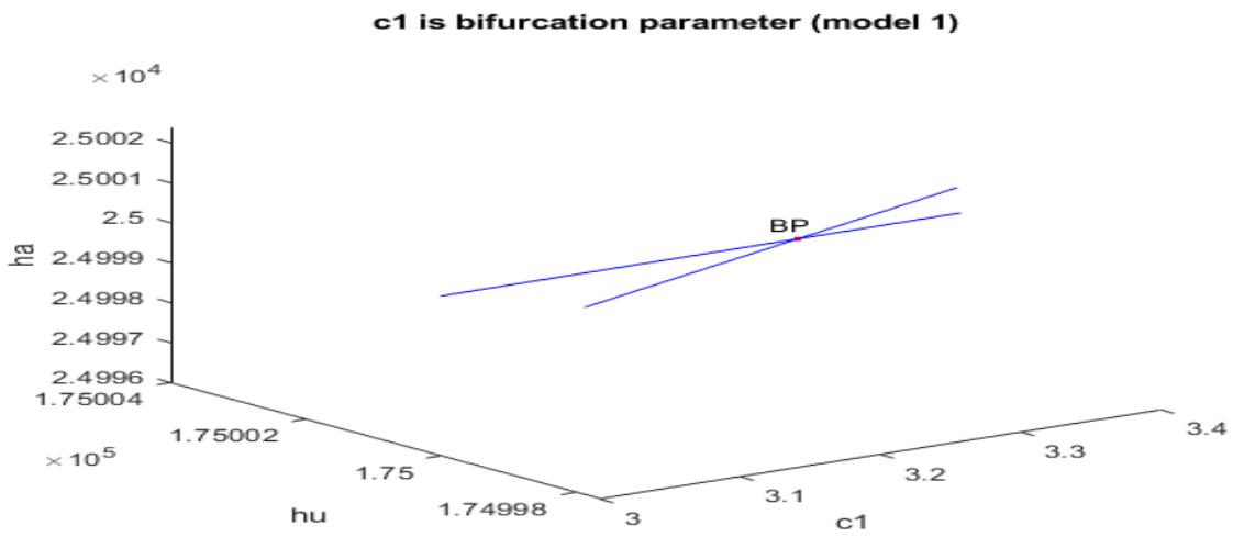RESULTS AND DISCUSSION The bifurcation analysis for model 1, with c1 as the bifurcation parameter, revealed a branch point at (hu; ha; hi; vs; vi; mv; c1) values of (175000; 25000; 0; 82918.739635; 0; 1; 3.255054) (Fig. 1a). For the MNLMPC calculations, hu (0) is set to 100000; $\sum_{t_i = 0}^{t_i = t_f}ha(t_i)$ were maximized and resulted in a value of 200000 and $\sum_{t_i = 0}^{t_i = t_f}hi(t_i)$ was minimized and resulted in a value of 0. The overall optimal control problem will involve the minimization of $(\sum_{t_i = 0}^{t_i = t_f}ha(t_i) - 200000)^2 +(\sum_{t_i = 0}^{t_i = t_f}hi(t_i) - 0)^2$ was minimized subject to the equations governing the model. This led to a value of zero (the Utopia point). The MNLMPC values of the control variables, c1, c2, and c3 were 0.5004, 0.5072, and 0.6403. The various MNLMPC figures are shown in figures 1b-1i. The control profiles c1, c2, c3 (Fig. 1h) exhibited noise, and this was remedied using the Savitzky-Golay filter to produce the smooth control profiles c1sg, c2sg, and c3sg (Fig. 1i). It is seen that the presence of a branch point is beneficial because it allows the MNLMPC calculations to attain the Utopia solution, validating the analysis of Sridhar(2024)[24]. The bifurcation analysis for model 2 with uo as the bifurcation parameter revealed a branch point at (sh; im; ic; rh; sv; iv;uo) values of (1000101.153725) (Fig. 2a). For the MNLMPC calculations, sh(0) is set to 0.7; $\sum_{t_i = 0}^{t_i = t_f}im(t_i),\sum_{t_i = 0}^{t_i = t_f}ic(t_i),\sum_{t_i = 0}^{t_i = t_f}iv(t_i)$ were minimized individually and each resulted in a value of 0. The overall optimal control problem will involve the minimization of $(\sum_{t_i = 0}^{t_i = t_f}im(t_i) - 0)^2 +(\sum_{t_i = 0}^{t_i = t_f}ic(t_i) - 0)^2 +(\sum_{t_i = 0}^{t_i = t_f}iv(t_i) - 0)^2$ was minimized subject to the equations governing the model. This led to a value of zero (the Utopia point). The MNLMPC values of the control variables, u0, u1 were 0.3778 and 0.3899. The various MNLMPC figures are shown in figures 2b-2i. The control profiles u0, u1 (Fig. 2h) exhibited noise, which was remedied using the Savitzky-Golay filter to produce the smooth control profiles uosg, u1sg. (Fig. 2i). It is seen that the presence of a branch point is beneficial because it allows the MNLMPC calculations to attain the Utopia solution, validating the analysis of Sridhar(2024)[24]. In both models, the presence of a branch point is beneficial because it allows the MNLMPC calculations to attain the Utopia solution, validating the analysis of Sridhar(2024)[24]. # VII. CONCLUSIONS Bifurcation analysis and multiobjective nonlinear control (MNL MPC) studies in two malaria transmission models. The bifurcation analysis revealed the existence of branch points in both models. The branch points (which cause multiple steady-state solutions from a singular point) are very beneficial because they enable the Multiobjective nonlinear model predictive control calculations to converge to the Utopia point (the best possible solution) in the models. A combination of bifurcation analysis and Multiobjective Nonlinear Model Predictive Control (MNL MPC) for malaria transmission models is the main contribution of this paper. # ACKNOWLEDGEMENT Dr. Sridhar thanks Dr. Carlos Ramirez and Dr. Suleiman for encouraging him to write single-author papers. Data Availability Statement All data used is presented in the paper. Conflict of interest The author, Dr. Lakshmi N Sridhar has no conflict of interest.  Fig. 1a: Bifurcation analysis of model 1  Fig. 1b: MNLMPC model 1(hu vs t)  Fig. 1c: MNLMPC model 1(ha vs t)  Fig. 1d: MNLMPC model 1(hi vs t)  Fig. 1e: MNLMPC model 1(vs vs t)  Fig. 1f: MNLMPC model 1(vi vs t)  Fig. 1g: MNLMPC model 1(mv vs t)  Fig. 1h: MNLMPC model 1(u1,u2,u3 vs t)  Fig. 1i: MNLMPC model 1(u1sg,u2sg,u3sg vs t) u0 is bifurcation parameter (model 2)  Fig. 2a: Bifurcation analysis of model 2  Fig. 2b: MNLMPC model 2(sh vs t)  Fig. 2c: MNLMPC model 2 (im vs t)  Fig. 2d: MNLMPC model 2 (ic vs t)  Fig. 2e: MNLMPC model 2 (rh vs t)  Fig. 2f: MNLMPC model 2 (sv vs t)  Fig. 2g: MNLMPC model 2 (iv vs t)  Fig. 2h: MNLMPC model 2 (control profiles noise exhibited)  Fig. 2i: MNLMPC model 2 (control profiles noise eliminated)

Generating HTML Viewer...