Coupling of CO2 Emissions and Economic Growth Across the U.S. between 2010 and 2015

I. INTRODUCTION

Mitigating global climate change through reduction of greenhouse gas emissions is a challenge of increasing urgency. It is a particular challenge because of the current fundamental interdependence of greenhouse gas emissions with economic production and human development. The primary cause of anthropogenic global climate change is the emission of greenhouse gases (GHGs), most importantly carbon dioxide from fossil-fuel combustion and other industrial processes [1]. A decoupling of emissions and the economy, as represented by the Gross Domestic Product (GDP), needs to occur to achieve the global aspirations of combating climate change [e.g., 1, 2, 3]. However, as Haberl et al. [4] note, shifting to renewable energy while sustaining current rates of economic growth may not solve the problem, and "meeting the goals of the Paris Agreement will require new and more effective policies than those deployed so far."

Reducing greenhouse gas emissions and achieving a low carbon economy will likely involve a reorganization of the patterns and scales of human activity. emissions per unit of value added ( ) provides a simple measure to explore this transition. Exploring this measure of decoupling emissions across time and space can provide insights to help guide understanding and decision-making.

While combating climate change has been a global priority for decades, progress on international and national public policy has moved slowly. This has driven subnational actors (such as cities, counties, and provinces), as well as non-state actors (such as corporations and non-government organizations) to enact their own policies to reduce their carbon footprints [e.g., 5, 6]. It is apparent that relevant and important decision-making occurs at multiple scales. It is also apparent that current broad differences, including inequities between and within countries, provide different incentives and opportunities for improvement among different demographics. Although has been mostly explored at the national level, there is a need to consider subnational variability to understand both national and within-country dynamics of the goals and their pursuit. National indicators may mask strong subnational differences, differences that may be meaningful in several ways - such as understanding the spatial disaggregation of national economies or identifying local challenges, 'successes,' 'failures,' inequities, and/or motivations. There is much insight to be gained by examining the sub-national scale. The linkage of emissions and GDP, and their evolution over time at a sub-national scale, should begin to reveal important elements of difference, including equity and social justice.

Products and data are now available to leverage multi-scale earth observations to evaluate indicators such as at the national level, but additional tools are needed at the subnational scale to inform regional and local decision makers. This paper explores the subnational distribution of decoupling greenhouse gas emissions in the United States (U.S.) over the period 2010 to 2015. We focus on the U.S. due to the availability of multiple-scale data on emissions and GDP. The period 2010 to 2015 is admittedly a short period and yet it provides an opportunity to examine the subnational character of changing directions in and GDP. Using the indicator we identify eight potential patterns of change over time (which we call cases) and investigate where each case was observed. Insights are provided on the sources of emissions and changes in GDP for areas experiencing each case. In section 2 we discuss how we derive our cases, our sources of data, and some key issues of data processing. In section 3 we describe the variability in decoupling at the state and county scales. Section 4 discusses some factors related to this variability and section 5 draws some brief conclusions.

II. MATERIALS AND METHODS

2.1. Decoupling GHG emissions and economic growth - CO /GDP

Considering as a function of time we can explore changes in the ratio of two related functions, and :

Defining the proportional growth of each quantity as with units of [time] , the counterpart for Eq. 1 for proportional growth rates is

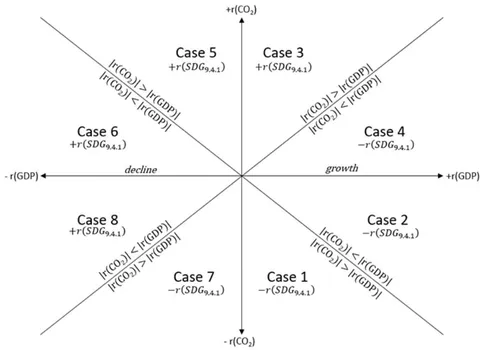
This allows us to categorize changes of into eight specific cases (see Table 1 and Figure 1). These 8 cases are defined by the rate and direction of change for , , and ; where is defined by the directions and relative magnitudes of and . Ideally decreases over time - i.e. there is a decrease in the amount of emissions per unit of economic output. This may or may not involve continuing economic growth.

The Organization for Economic Co-operation and Development defines decoupling as "breaking the link between 'environmental bads' and 'economic goods'," specifically when "the growth rate of an environmental pressure is less than that of its economic driving force (e.g., GDP) over a given period." Thus, when is decreasing, decoupling is occurring (cases 1, 2, and 4 below). Haberl et al. further distinguish between absolute and relative decoupling: "GDP growth coinciding with absolute reductions in emissions or resource use is denoted as 'absolute decoupling' as opposed to 'relative decoupling', where resource use or emissions increase less so than does GDP." By focusing on we identify a fourth case of decoupling, case 7, where both emissions and GDP are decreasing, but emissions are decreasing faster. Cases 3, 5, 6, and 8 are then classified as "not decoupling" as they are not seeing a decrease in the ratio of to GDP over time. Shan et al. have used a similar analysis to examine decoupling of emissions and GDP for cities in China. The IPCC similarly distinguishes between absolute and relative decoupling. Our cases 1, 2, 4, and 7 all have negative values of , and all qualify as decoupling, but the distinctions in terms of the relative values for the changes in and GDP are important and we carry forward the distinctions. Likewise, cases 3, 5, 6, and 8 all qualify as not decoupling but we preserve the important distinctions.

Table 1 and Figure 1 show that there are multiple paths to decreasing . Absolute decoupling occurs when emissions decrease while GDP increases, cases 1 & 2. Relative decoupling occurs in other cases where the change in is negative (i.e. more GDP per unit of ), in case 4, where emissions are still increasing but at a decreasing rate with respect to GDP, and in case 7 where the economy is in decline, but emissions are declining faster than GDP. Not decoupling likewise occurs in several combinations. In case 3 the economy is growing, but at the cost of increasing emissions. Cases 5 and 6 are in economic decline despite increasing emissions. Finally, in case 8, both GDP and emissions are declining but GDP is declining faster so that the change in is positive and decoupling is not occurring. Table 1 provides a vocabulary to characterize and discuss the eight cases.

Table 1: The direction and relative magnitude of changes in emissions and GDP define eight cases for the pattern of changes in . The last column defines the vocabulary for discussing the eight cases in this paper. See also Figure 1.

Figure 1: A Cartesian diagram of the eight cases defined in Table 1, where the x-axis is the change in GDP, r(GDP), and the y-axis is the change in emissions . The diagonal lines separate whether r(GDP) or has the greater proportional rate of change (the 'dominant' rate). See also Table 1.

2.2. Data on emissions

Data are available on national-level emissions from multiple sources. For example, the CDIAC-FF estimates of emissions from fossil fuel combustion and cement manufacture provide annual, global measures of anthropogenic from all countries for the time period 1751-2020 [10]. Other datasets also provide recent national-level estimates, but with slightly different boundaries of what is or is not included. Datasets may, for example, not include emissions from cement manufacture [11] or may include additional industrial sources of [12]. With different system boundaries possible it is important that comparisons across countries or across time use consistent system boundaries for the accounting.

For our analyses at the level of U.S. states we use emissions estimates from the U.S. Energy Information Administration for the years 2010-2015 [11]. The EIA obtains emissions estimates based on fuel type (coal, natural gas, petroleum) and does not include emissions from cement manufacture. We have adjusted the state data to account for the difference of the total sum of emissions from all states and the national estimate. The emissions estimates are from direct fuel use from all sectors (residential, commercial, industrial, and transportation). The U.S. does not provide uncertainty values for the state-level emissions data, but it is generally expected to be comparable to or slightly larger than the uncertainty of the national estimates which is reported at -2 to +4%.

To estimate county-level emissions, we aggregated data from the Vulcan version 3.0 dataset [13], which provides 1 km x 1 km hourly emissions estimates for the United States for the years 2010-2015. Emissions are categorized into ten source sectors and allow us to examine sectoral details to better understand the heterogeneous patterns at the county level: residential, commercial, industrial, electricity production, on-road, non-road, commercial marine vessel, airport, rail, and cement manufacture. For the benefit of graphic display, we have focused on the contiguous U.S. states. The critical Vulcan data that allow construction of emissions estimates at the county level are only available for the 2010-2015 interval. The Vulcan estimates of emissions are based on multiple data sources, each with its own uncertainty, so uncertainty at the county level will vary with the mix of emission sources, and uncertainty at the national level is estimated at +/- 8% (13). The state-level Vulcan data are compared to sector and fuel-specific data in the EIA datasets, and the county-level emissions data are believed to be sufficiently certain to support meaningful conclusions.

We utilize different datasets at different scales to emphasize exploring the construct validity of and its eight cases as a useful tool over conserving the numerical consistency across spatial scales. We thus make use of the high accuracy of EIA data at the state level, as well as the analytic freedom afforded by the detailed, sectoral Vulcan data for the county level. Emissions from cement manufacture (which constitute less than 1% of U.S. emissions) are thus not included in the state data. While this affects the numerical values of , it has a negligible effect on our area of interest - patterns and trends.

2.3. Data on Economic Output (GDP)

For the U.S., the Department of Commerce, Bureau of Economic Analysis (BEA) maintains data on GDP at the state and county levels. An advantage of confining this analysis to the U.S. is the detailed, multi-scale, spatially-explicit data available on GDP and hence the avoidance of having to derive estimates from national or regional data or assumptions on per capita values.

2.4. Methods and Data Processing

Our county level analysis combined Vulcan 3.0 CO emissions data with county-level GDP data from the BEA. Because Vulcan 3.0 quantifies CO emissions at a resolution of 1 km x 1 km per 1 hour, analysis within a geographic information system was used to convert the data to the county and annual level. The complete Vulcan 3.0 dataset was downloaded from the Oak Ridge National Laboratory Data Archive Center. A county boundary shapefile was acquired from the 2019 U.S. Census Bureau TIGER/Line County data file [15]. Both the Vulcan raster files and U.S. County shapefile were imported into Esri's ArcGIS Pro [16]. The projection of the U.S. County boundaries shapefile was reprojected to the Lambert Conformal Conic 2SP to match the Vulcan 3.0 georeferencing system. Using the Spatial Analyst tool Zonal Statistics as Table [17], the CO emissions estimates were calculated and summarized within the county boundaries provided by the U.S. County boundaries shapefile and reported as a table. Each table contains 3108 records, the total number of counties and county equivalents in the conterminous United States (including 38 independent cities in Virginia). This process was repeated for each of the 6 Vulcan years, as well as for each economic sector.

A table was also created in R for the rates of change for both states and counties. This table derived the proportional growth rates for , GDP, and with units of inverse years. This was implemented in the code by taking the log of the ratio between values for 2010 and 2015 for emissions and for GDP, which was then divided by five, the time span between the two years. For calculating the rates, the difference between the emissions rate and GDP rate was calculated as shown in Equation 2. The output was used to identify which case each state or county belonged in, based on the criteria in Table 1. The absolute and relative rates of change were calculated for the state and county level values. The relative change was determined by taking the 2015 value and dividing it by the 2010 value. The absolute change was calculated by taking the difference between the 2010 and 2015 values.

In this analysis the contiguous U.S. was taken to include 3080 counties and county equivalents, including ten of the independent Virginia cities that are not legally included in the counties in which they are geographically embedded (Alexandria, Chesapeake, Hampton, Newport, Norfolk, Portsmouth, Richmond, Roanoke, Suffolk, and Virginia Beach). All 28 of the other independent Virginia cities were processed with the appropriate counties. The District of Columbia was treated as a state comprised of one county.

III. RESULTS

3.1. Decoupling emissions and economic growth: changes in in the United States at the state level While is often reported as a national aggregate, we focus on the substantial differences found at the state and at the county level in the United States [see also 18]. To track changes over time we focus on the period 2010-2015 as this time interval is supported with the high-resolution VULCAN 3.0 emissions dataset [13].

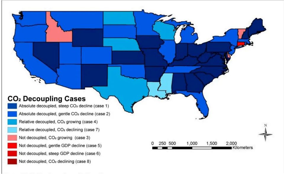
Although the majority of U.S. states (including the District of Columbia, which is absolute decoupling with steep decline (case 1), have shown absolute decoupling of greenhouse gas emissions and GDP (cases 1 and 2), with decreasing and increasing GDP (Figure 2 and Table 2), there were 8 states with increasing emissions over the 2010 to 2015 period. Delaware had the fastest rate of growth in both emissions and . Four states (Louisiana, Connecticut, Mississippi, and Alaska) had decreasing GDP during this time period. The cases of not decoupling with declining (case 8) and not decoupling with steep GDP decline (case 5) were not observed at the state level and only in Connecticut did emissions increase while GDP decreased (case 6).

Georgia showed the fastest rate of increasing GDP and the fastest rate of decreasing . States decoupling with steep decline were the source of an increased fraction of U.S. total emissions despite their decreases in absolute total emissions. Almost 80% of U.S. emissions came from states with increasing GDP and declining emissions (cases 1 and 2).

Table 2: The 50 U.S. states and the District of Columbia are classified according to the eight cases described in Figure 1 and Table 1, and for each case the total of emissions as a fraction of U.S. total emissions for the relevant states is shown for 2010 and 2015. data are from the U.S. EIA [11] and GDP data are from the U.S. Bureau of Economic Analysis [14].

Figure 2: State level mapping of the different cases of for the contiguous U.S. states and the District of Columbia. Each state is indicated according to the 8 cases identified for the period 2010 to 2015. Not shown: Alaska is relative decoupling with declining (case 7), Hawaii is absolute decoupling with gentle decline (case 2), and the District of Columbia is absolute decoupling with steep decline (case 1). Cases 1, 2, 4 and 7 (blue) had decreasing while cases 3, 5, 6, and 8 (red) had increasing . data are from the U.S. EIA [11] and GDP data are from the U.S. Bureau of Economic Analysis [14].

3.1. Decoupling emissions and economic growth: changes of in the United States at the county level

At the county level the spatial distribution of cases was complex, with all 8 identified cases represented for the period 2010 to 2015. Approximately one-third of counties in the contiguous United States had growing economies with absolute decoupling of emissions and GDP (cases 1 and 2, see Table 3) - whereas almost 80% of the U.S. states exhibited this absolute decoupling (Table 2). Counties with relative decoupling (cases 4 and 7) comprised another one-third of counties and counties not decoupling (cases 3, 5, 6, and 8) comprised the final one-third of counties. Approximately 14% of counties had emissions rising despite a declining economy (cases 5 and 6). While 84% of the contiguous states had declining emissions, only 53% of the counties did. This shows that national and state-level decreases in emissions masked widespread local increases (47% of all counties). Those counties with declining emissions (cases 1, 2, 7, and 8) represented 65.8% of emissions from the contiguous U.S. in 2010, and 59.3% in 2015. The counties with decreasing emissions had a gross decrease in emissions of 162.4 Mt between 2010 and 2015. The cases with increasing emissions represented a gross increase of 69.3 Mt C, leading to a net decrease of 93.1 Mt C in the contiguous United States.

Table 3: The contiguous U.S. includes 3080 counties and county equivalents, with representatives of all 8 cases for the changes in from 2010 to 2015 described in Table 1 and Figure 1. The portions of emissions for the contiguous U.S. are shown for 2010 and 2015. The District of Columbia is treated as a state comprised of a single county. data are from Gurney et al., [13], and GDP data are from the U.S. Bureau of Economic Analysis [14].

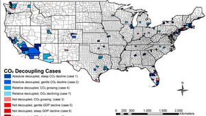
The geographic distribution of the cases at the county level is presented in Figure 3. At this scale all 8 cases appeared broadly across the country. Recognizing that we use different sources for estimates of emissions data at the state and county levels, it appears that even for states that were characterized as undergoing absolute decoupling with growing economies, such as Iowa, North Carolina, and West Virginia, each of the 8 cases appeared for counties within them. Texas (relative decoupling with growing - case 4) and Mississippi (relative decoupling with declining - case 7) also included counties with all 8 cases. Even though there was only one state with growing emissions despite decreasing GDP (cases 5 and 6) (Connecticut), there were over 430 counties nationally with these changes. In some states, a small number of counties with large economies dominated the state-level trend, such as in Chittenden County in Vermont and New Castle County in Delaware, both of which were not decoupling, growing economies (case 3).

Figure 3: County level mapping of the different cases of decoupling for the contiguous U.S. states and the District of Columbia. Each county is indicated according to the 8 cases identified for the trend in for the period 2010 to 2015. Cases 1, 2, 4 and 7 (blue) had decreasing values for while cases 3, 5, 6, and 8 (red) had increasing values for . data are from Gurney et al [13] and GDP data are from the U.S. Bureau of Economic Analysis [14].

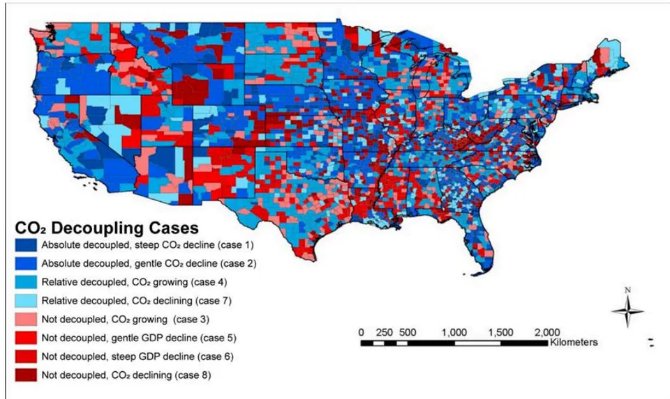
Table 4 summarizes the cases in terms of average values and relative annual changes in emissions. For the time period 2010 to 2015 counties characterized as not decoupling with growing and not decoupling with gentle GDP decline (cases 3 and 5) showed, on average, the largest relative increases in emissions, at 4.49 and 3.28%/year respectively. Counties with relative decoupling with declining (case 7) had the largest relative decreases in emissions, at 4.94%/year, followed by counties with absolute decoupling and steep decline (case 1), at 3.92%/year. Counties from cases 1 and 7 were also the counties with the largest absolute values for average emissions. With both of these classes of counties decoupling, this suggests that decoupling in the U.S. as a whole was being driven in significant measure by reducing the emissions from high-emitting counties.

Table 4: Average values for emissions and average annual rate of change in emissions for all counties in each of the 8 cases. The time interval represented is 2010-2015. Primary data are from Gurney et al. [13].

IV. DISCUSSION

Having observed the subnational variation in changes of , we explore some of the characteristics of the eight different cases identified. We suggest that understanding the causes of subnational variability in decoupling of emissions and economic growth is important to understanding our ability to achieve sustainability at a global level. We make a first attempt at exploring this in the U.S. by looking at decoupling at the county level and some of characteristics of the different cases of decoupling, including the sources of emissions by economic sector, the rural-urban continuum, and the concentration of population.

4.1. CO Emissions at the county level by economic sector

Figure 4 shows the average magnitude of emissions from each economic sector for 2010 and 2015, for each of the eight cases of decoupling. Table 5 shows the average emissions change in each sector for each case as a percent and as total megatons of C (MtC). Together Figure 4 and Table 5 show, for example, that for the set of counties with absolute decoupling with steep decline (case 1), on average, electrical production was the dominant source of emissions (with over 50% of the total in both 2010 and 2015) and that emissions from electrical production declined by 28% from 2010 to 2015. Similarly, in the set of counties with absolute decoupling with gentle decline (case 2), on average, on-road emissions were the largest contribution, contributing 35% of emissions in each year while declining by 1.1% from 2010 to 2015. On-road emissions increased in counties with relative decoupling with growing and in counties not decoupling with growing (cases 3 and 4). Whether electricity production or on-road emissions was the dominant contribution to emissions has generally defined whether r(GDP) or r( ) was the dominant factor in the 2010-2015 change in .

Overall, the sector contributing the most to decreases in emissions was electricity generation, with a total reduction of 91.9 Mt C from 2010 to 2015. Commercial marine vessels (cmv) were a distant second with a total 10.1 Mt C decrease, however cmv had by far the largest percent change, at -40% from 2010-2015, with rail the second largest percent change at +24%. emissions from electricity production, while experiencing the greatest decreasing change, remained the largest source of emissions. The second largest source of emissions, on-road, saw relatively little change from 2010 to 2015. In cases where was the principal driver of change (cases 1, 3, 5, and 7), whether decoupling or not, electricity production was the largest source of emissions. Where on-road emissions were the dominant source, was not the dominant factor in changing . In cases where on-road emissions were the dominant source of emissions, GDP was the principal factor in the evolution of (cases 2, 4, and 6). The exception was where there was not decoupling despite declining (case 8), where electricity production was the major source of emissions but GDP was the dominant factor in driving the change in (case 8). Almost by definition, most of the emission reductions occurred in counties with absolute decoupling with steep decline or with relative decoupling with declining (cases 1 and 7).

Airport, commercial, and rail-related emissions went up, on average, in all cases (with a few exceptions), and residential emissions went down in all cases, which suggests that changes in these sectors are occurring nationwide irrespective of local trajectories in decoupling. The largest increases in emissions were from the commercial sector - notably in three of the four cases with increasing GDP (cases 2, 3 and 4) - although the only case with negative values for the commercial sector was for counties with absolute decoupling with steep decline (case 1). Industrial sector emissions increased in counties not decoupling with growing and relative decoupling with growing (cases 3 and 4) counties while decreasing notably in counties with absolute decoupling with steep decline and relative decoupling with declining (cases 1 and 7). Industrial sector emissions increased by smaller amounts in case 5 and 6 counties while decreasing in case 2 and 8 counties. The industrial sector is perceived as hard to decarbonize and the energy mix has remained relatively unchanged (see [19] and [1]).

In sum, the set of counties with increasing total emissions of from 2010 to 2015, on average, (cases 3, 4, 5, and 6) had increases from both the electric power and industrial sectors while the set of counties with decreasing total emissions (cases 1, 2, 7, and 8) had, on average, decreases from both the electric power and industrial sectors. Note that some of the decrease in emissions per unit of electricity generated was offset by increases in total electrical production, especially in case 3 counties (not decoupling with growing). However, change in electrical production was still the driving factor in transitioning toward a lower carbon economy [20]. Electricity generation highlights the linkages among counties. Although the emissions from the generation will be accounted in one county the product power can be employed in nearby counties. The same is true for emissions from industrial facilities in that the products can be widely employed outside of where the emissions occur. What is being observed now is the availability of technologies to produce electricity with lower emissions.

{"image_source":{"path":"images/1425c81c4f8939d686ca025630d1ac3a28e0f1233bd09ac528b1d60338ad87a5.jpg"},"content":"","chart_caption":,"chart_footnote":[]}

Table 5: Average change in the percentage and in the magnitude of emissions (in megatons carbon) by case and sector for U.S. counties from 2010 to 2015. Summing across the table rows of the total of emissions does not always agree due to rounding. Columns indicate whether decoupling was taking place. CMV is commercial marine vehicles.

4.2 The rural-urban character of counties for the eight cases of decoupling

A striking observation of the analysis displayed in Figure 3 is the spatial heterogeneity in the pattern of changes in decoupling over time. The eight cases for change in were all widely observed and the various cases were observed within a single state and among adjacent counties. These variations reflect the spatial disaggregation of the national economy and have the potential to identify differences in economic activity, local inequities, and/or local motivations for addressing the need to decrease emissions. The complex heterogeneity reflects intercounty transfers of electricity and of manufactured and agricultural products. It reflects differences in wealth, resources, and opportunity. Over time it will show efforts to combat climate change and how the opportunities, motivations, and cost of mitigating climate change are spatially distributed. We ask whether some of the diversity is related to urban-rural differences and the structure of urban areas.

The rural-urban character of our eight cases (Table 6) is expressed here through the Rural-Urban Continuum Codes (RUCC) of the U.S. Department of Agriculture (see Endnote 1). The RUCC is a classification scheme that distinguishes counties between "metro" (metropolitan) and "non-metro" and classifies metro counties by the population size of the metropolitan area it is a part of and non-metro counties by the degree of urbanization and the adjacency to a metro area. Code 3 to code 4 marks the transition from metro to non-metro counties. The RUCC classification captures both a county's population and the influence of adjacent metro areas, which can be important when considering local drivers of emissions and GDP. Note that the numbering of non-metro counties alternates between metro-adjacent and non-adjacent as population lowers. Like our decoupling case numbers, RUCC codes are descriptive, not indications of magnitude. RUCC 1 is a county in a metro area of over one million population, RUCC 9 is a county that is completely rural or with population under 2,500.

All eight of the cases were found in all nine rural-urban settings. All RUCC codes (except 5) had their highest frequency in cases of absolute decoupling with gentle decline or relative decoupling with growing (cases 2 and 4), the most commonly occurring cases. There is no obvious relationship (Table 6) between rural character and decoupling of emissions from economic growth, although 80% of the largest urban areas (RUCC = 1) were decoupling. While there are concentrations one cannot assume, for example, that rural areas consistently exemplified a particular per GDP relationship.

Table 6: The relationship between urban-rural character and the case for U.S. counties, shown as the number of counties in each category. Rural-urban character is according to the RUCC of the U.S. Department of Agriculture (see text and Endnote 1). Columns indicate whether or not decoupling was taking place.

4.3 County population concentration and the eight cases of decoupling

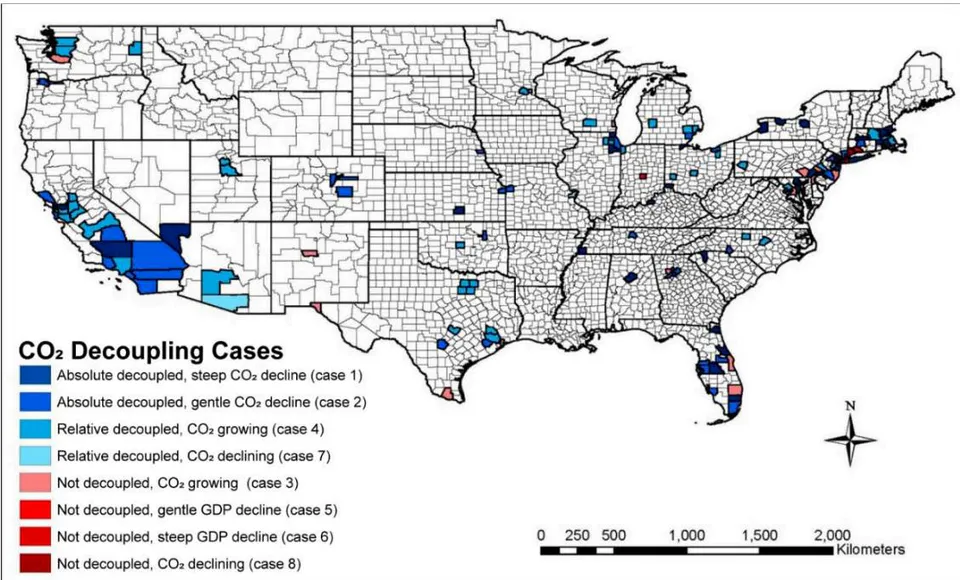
Half of the U.S. population lived in only 146 of the 3080 counties in our study (see Figure 5), meaning that trends and relative changes in do not tell the full picture when giving equal weight to every county in the contiguous U.S. The circumstances in these 146 counties do tell the circumstances under which half of the U.S. population was living. Of these 146 counties, only 8 (5%) had decreasing GDP (compared to of all counties) and only 20 (14%) had increasing (compared to of all counties). This suggests that large urban areas were indeed disproportionately driving decoupling in the U.S., a potentially important linkage in the relationships among urbanization, population, GDP, and emissions.

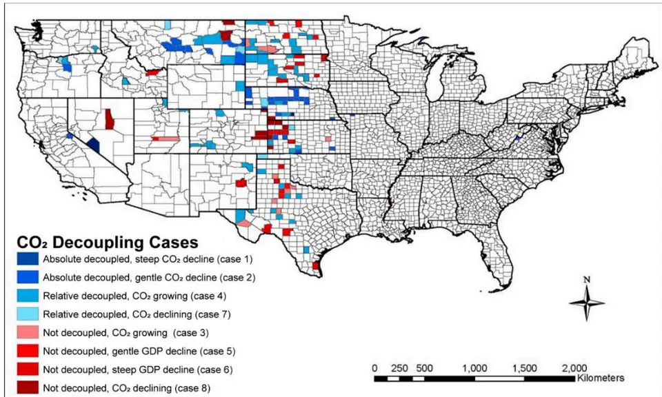
For contrast, Figure 6 shows the decoupling case for the 146 least populous counties. Of these counties 46 (32%) had decreasing GDP and 51 (35%) had increasing, both percentages typical of the country as a whole.

Figure 5: The case for the most populous 146 counties in the U.S. These counties collectively encompassed 50% of the U.S. population. These 146 counties represented only 4.7% of the counties included in this analysis and were all, except one, RUCC category 1. Not shown, Honolulu County in Hawaii, which is absolute decoupling with gentle decline (case 2). data are from Gurney et al. [13], GDP data are from the U.S. Bureau of Economic Analysis [14], and population data are from the U.S. Census Bureau [22]. Figure 6: The case for the least populous 146 counties in the U.S. In contrast to Figure 5, these 146 counties encompass 0.08% of the U.S. population. data are from Gurney et al. [13], GDP data are from the U.S. Bureau of Economic Analysis [14], and population data are from the U.S. Census Bureau [22].

V. CONCLUSIONS

This study provides a context to characterize the changing relationship and broad heterogeneity in the nature of decoupling between emissions and GDP in the United States over the years 2010 to 2015. Sustainable Development Goal Indicator 9.4.1, , was adopted by the UN [23, 24] in order to examine and monitor the decoupling of emissions and economic development at the national level but use at the national level (which shows decoupling in the U.S.) risks missing the insights that are revealed when we examine the indicator at subnational scales. Even at the state level in the U.S. suggests homogeneity as 46 states and the District of Columbia showed decoupling of emissions and GDP for the period 2010 to 2015. Only eight states showed increasing emissions. To the contrary, whereas emissions over the 2010 to 2015 interval were reduced broadly, largely from electric power generation, the decoupling of emissions and economic development varied widely when examined at the county level. Whereas 90% of states showed decoupling of emissions, only 65% of U.S. counties had decoupling of emissions and GDP.

We have defined eight cases to characterize the changing relationship between the magnitude and direction of changes of emissions and GDP and we show that all eight cases prevail in counties across the country and across the rural-urban landscape. Of 3080 counties and county equivalents in the conterminous U.S., 1024 counties showed an increase in GDP with a decrease in emissions for the period 2010 to 2015 (absolute decoupling, our cases 1 and 2). In another 625 counties emissions decreased but GDP decreased as well (cases 7 and 8).

Approximately one-third of U.S. counties were not decoupling emissions from economic growth over the period 2010 to 2015. The data show that decoupling emissions from economic growth was very sector specific and dominated by the electrical generating sector. Many counties with large contributions from electrical generation were experiencing declining emissions with continuing economic growth (cases 1, 2, and 4). Counties with rapidly growing emissions from the electrical, industrial, and other sectors were not decoupling whether GDP was growing (case 3) or declining (case 5). Of counties with declining GDP, 431 had emissions increasing (cases 5 and 6) while 625 had emissions declining (cases 7 and 8).

On average, counties in three of our four cases of decoupling were characterized by decreasing emissions from the electricity sector. For cases with decreasing emissions there were decreasing emissions in both the electrical and industrial sectors. If emissions were growing there was growth in both the industrial and electrical sectors and three of the four cases of not decoupling were characterized by increasing emissions sources in both the electrical and industrial sectors. High emitting counties tended to be decoupling emissions from economic growth and reducing emissions. But the heterogeneity was widespread. States that showed absolute decoupling of emissions from economic growth still contained counties with increasing emissions and economic decline.

The challenge going forward is to balance economic growth and emissions. Decoupling now largely reflects changes in the electrical sector and the electrical sector provides services that extend beyond county boundaries. The needed reductions in emissions will require emissions reductions from the broader economy and carry the risk that reductions in one place are offset by increases elsewhere. The rise in electric transportation could create such a circumstance as emissions from road transport decrease in one county while emissions from electrical generation in another county are stable or increasing. Neither climate goals nor social equity are served by relocating emissions sources across counties, states, or countries.

Although we did not show a systematic relationship between decoupling and rural/urban character, for the 124 counties that were home to half of the U.S. population was decreasing in 86%. The most striking feature of our characterization of decoupling is the heterogeneity observed at county-level spatial resolution. If a significant decrease in reliance on emissions is to occur for the U.S. it will have to involve more geographic areas and have a greater involvement across economic sectors.

2013 Rural-Urban Continuum Codes Endnote: Rural-Urban Continuum Codes from the U.S. Department of Agriculture [21]

Author Contributions: Conceptualization, A.B., J.C., C.D., C.F., N.G., D.G., and G.M.; methodology, A.B., J.C., C.D., C.F., N.G., D.G., and G.M.; software, A.B., C.D., C.F., and N.G.; validation, A.B., C.D., C.F., and N.G.; formal analysis, A.B., J.C., C.D., C.F., N.G., D.G., and G.M.; data curation, A.B., C.D., C.F., and N.G.; writing-original draft preparation, J.C., D.G., and G.M., writing-review and editing, A.B., J.C., C.D., C.F., N.G., D.G., and G.M.; visualization, A.B., C.D., C.F., and N.G.; project administration, J.C., D.G., and G.M. All the authors have read and agreed to the published version of the manuscript.

Funding: This research received no external funding.

Acknowledgments: We thank the Research Institute for Environment, Energy, and Economics (RIEEE) at Appalachian State University for providing funding for this research.

Conflicts of Interest: The authors declare no conflicts of interest.