‘Discrete Maximum Principle Honored by Conventional Finite Volume Schemes for Diffusion-Convection-Reaction Problems: Proof with Geometrical Arguments

I. INTRODUCTION

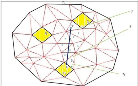
Let be a bounded connected open subset of whose boundary denoted by is the union of polygonal lines where is a finite subset of which denotes the set of positive integers (see Figure 1 below). Note that if is a singleton then is a polygon (and so simply connected). Given the scalar functions , and together with a vector field , all being defined in , we consider the elliptic problem that consists in finding a scalar function in an adequate function space such that

with the following homogeneous Dirichlet boundary conditions:

Under reasonable assumptions on the previous data i.e.

with

it is easy to prove that (see [1] for instance): The second order elliptic problem (1.1)-(1.2) gets a unique weak solution in the sense that

where we have set:

and

Following [2] one can prove that if the given function is positive almost everywhere in then the weak solution of the system (1.1)-(1.2) is also positive almost everywhere in . That is the weak form of the Maximum Principle. Several works on construction of positivity-preserving numerical methods for diffusion, diffusion-convection, diffusion-reaction and diffusion-convection-reaction problems are available in the literature (see for instance [5, 6, 11, 13]). Such numerical methods are sometimes called monotone schemes.

The main objective of this work is to expose geometrical arguments for proving the well-known discrete version of the Maximum Principle satisfied by the conventional finite volume solution to the system .

II. PRELIMINARY TOOLS

Definition 2.1 (Partition of ). Let be the closure of in the sense of the standard topology of and let be a finite subset of which is the set of positive integers. A family made up of subsets of defines a partition of if the following conditions are satisfied:

where denotes the interior of in the sense of standard topology of .

Let us consider a partition P over consisting in a finite family of closed convex polygons (named also polygonal elements) generically denoted by T. These polygonal elements are the so-called control volumes in the language of Finite Volume theory. The control volumes from the partition P defines a conforming Finite Volume mesh over if (in addition to conditions (i)-(iii) from Definition 2.1) the following conditions are satisfied:

where denotes the empty set. Let us denote by the set of boundary edges (viewed as degenerate control volumes) and we briefly define the conventional finite volume mesh T as it follows: .

We should use intensively in what follows a notion of characteristic function slightly different from the usual one and defined as follows.

Definition 2.2 Let T be a control volume either from P or from . We call in this work the characteristic function of T denoted by the function defined almost everywhere either in (with respect to Lebesgue measure in 2-D) or on (with respect to Lebesgue measure in 1-D) by:

where denotes the exterior of a subset from (with respect to the natural topology of ). Recall that stands for the interior of from . ☐

Let us introduce the following discrete function spaces that play a key-role in the sequel.

Definition 2.3 We set:

where is the zero-function (denoted simply 0 if there is no risk of confusion) from the discrete function space . ☐

The Finite Volume method is based on the fundamental idea that the exact solution u could be approximated inside any control-volume T with a constant corresponding to either the mean-value of u or its approximation at a given point located inside T, with Cartesian coordinates . In the context of conventional Finite Volumes the choice of that point is not arbitrary as we will be seeing in assumption below. Let us denote by the boundary of any control-volume T. We need to specify the following assumptions that make the conventional Finite Volumes very attractive and realistic for certain engineering problems as subsurface flow problems (notice that [3, 4, 15] are among distinguished references on fluid flow in porous media):

The diffusion coefficient is a piecewise constant function i.e.

where defines a partition of the domain in the sense of Definition 2.1.

Denote by T the Finite Volume mesh corresponding to the partition P. Let us make the following assumption on T.

is compatible with the discontinuities of in the sense that the discontinuity points of belong to the mesh interfaces , where we have set . In other words any discontinuity point of the function is located in a control volume boundary.

(A3) For all such that and are adjacent (that is is a common edge for control volumes and ), the vector is orthogonal to the common edge. This is the so-called orthogonality condition required for conventional Finite Volume meshes (see [5, 6]).

An immediate consequence of the assumption (1.3) is that is a nonnegative constant function in each control volume T. We denote by the constant value of in the control volume T.

Let us give a brief description of the different steps for getting a conventional finite volume scheme. We start with introducing some useful notations: E is the set of all mesh edges, is the subset of E made of interior mesh edges and is the subset of E made of exterior mesh edges i.e. mesh edges lying on the domain boundary.

Step 1: Integrate the two sides of the balance equation (1.1) in each control volume from the family . So we get what follows (thanks to Ostrogradski's theorem):

where stands for outward unit vector normal to the control-volume boundary .

Step 2: Re-write the first two integral terms from the left-hand side of (3.2) as follows for all :

where is the set of mesh edges lying in and where stands for outward unit vector normal to the portion of the control-volume boundary , called again mesh edge associated with . Integrals from the first summation are diffusion fluxes while integrals from the second summation are convection fluxes (called sometimes advection fluxes).

Step 3: Perform the approximation of the unknown function u in the control-volume T with the unknown real constant . So one could set what follows concerning approximation of the reaction term:

where is the integral of a function defined in the control volume T.

Step 4: Look for reasonable approximations of flux integral terms from the left-hand side of (3.3). What should one understand by reasonable approximations? We mean that the flux approximations should take account of the following constraints:

• Perform the upwind approximation of the convection flux in view to ensure the stability of the global finite volume scheme. For that purpose, let us start with setting:

Definition 3.1

Definition 3.2 (Upwind approximation of the convection flux over ) Let in , with T and L from the set P. We set:

In other words the upwind approximation of the convective flux across the interior edge in could be defined as follows:

Since (according to the flux continuity principle over grid-block interfaces)

the preceding approximation of the convective flux is equivalent to the following one

• The flux continuity across interior edges , i.e. , is a fundamental physical principle to be met. So we have necessarily for all

Integrating the right-hand and the left-hand sides of (3.9) over leads to the following "weak formulation" of flux continuity:

Since the weak solution of the system (1.1)-(1.2) lies in , the trace exists (in for instance) in a unique manner. In consequence we naturally get what follows:

Thus, the previous "weak formulation" of flux continuity (3.10) is reduced to

In the context of conventional Finite Volumes the family P satisfies the so-called orthogonality condition (see assumption above at the beginning of the current Section). So there exists a family of points , such that for any pair , with T and L adjacent, the orthogonal projections of and on their common edge coincides and let call it . We make the following convention:

"If is adjacent to the domain boundary we set: , where is the boundary edge associated with , and coincides with ".

This being said, from the following diffusion flux approximation (assuming the exact solution restriction in for any ; it is the case if ):

where stands for Lebesgue measure in one-space dimension, represents the Euclidean distance and where is in fact the point seen as from the boundary of T by an observer standing inside T. The principle of continuity of u on grid-block interfaces is expressed at the discrete level by the relation:

where is the subset of made of such that T and L are adjacent. So it is reasonable to set:

With the above notation the diffusion flux approximation could read as follows

Writing down the discrete analogue of the "weak formulation" (3.12) of continuity of the diffusion flux (across any interior edge ) yields

This relation could be viewed as a linear equation with only discrete unknown . This unknown can be obviously determined as a function of discrete unknowns and as indicated hereafter. Indeed elementary operations on (3.15) leads to

where we have set

Substituting the right-hand side of (3.16) to in the diffusion flux approximation given by (3.14) leads to what follows for any :

Remark 3.3 (Important to notice)

First of all the diffusion flux approximation (3.18) has been established for interior edges i.e. . Let us explain why the convention consisting to consider boundary edges as also degenerate control-volumes L allows to recover (3.14) from the relation (3.18). Indeed if then , and it follows that in (3.18).

The following Conventional Finite Volume scheme is obtained from preceding approximations of different terms of the left-hand side of the balance equation (3.3): see relations (3.4), (3.8) and (3.18). One could learn more on this topic with [5, 6] for instance.

Definition 3.4 (Conventional Finite Volume Scheme)

The conventional Finite Volume approximation of the system (1.1)-(1.2) consists in what follows:

Find

such that:

where . Recall that is the integral of a function defined in the control volume T. ☐

The Finite Volume and Mimetic Finite Difference approximations of solutions to isotropic or anisotropic diffusion problems on distorted grids have been intensively developed in the literature and are today considered as classical topics (see for instance . Some extensions of Finite Volume Methods have been designed and known under the name of Gradient Discretization Methods (see for learning more) and many other extensions are underdevelopment (see for instance). Let us state the following well-known Discrete Maximum Principle followed by a proof based upon a Geometrical Technique that seems new in this context to the best of our knowledge.

Theorem 3.5 (Discrete Maximum Principle) Let us suppose that is a bounded open subset of , connected by polygonal arcs. Let its boundary be the union of polygonal lines , where is a finite subset of (see Figure 1 below). The linear system (3.19) gets a unique solution that satisfies the following positivity property:

• If for all then

Moreover the following discrete maximum principle holds:

• If there exists a control volume from such that

then

The originality of this work relies up on the technique exposed hereafter to prove that the solution to meets the discrete Maximum Principle. This technique has been successfully applied to a new finite volume method introduced recently by A. Njifenjou, A. Toudna and S. Moussa in [11]. To the best of our knowledge the technique widely exposed in the literature (for proving the discrete maximum principle) is based up on algebraic arguments (see for instance ). We are going to develop geometric arguments for proving the discrete Maximum Principle stated above in Theorem 3.5.

IV. GEOMETRICAL TECHNIQUE FOR PROVING (3.20) AND (3.21)

◇ We have to first prove (3.20), that is:

If

with

then

Let us set for all :

. Then notice that if T and L are adjacent control volumes i.e. and get a common edge, we have

and otherwise we have

In the sequel denotes the set of control volumes from adjacent to a given control volume E from P.

Let us start the proof with assuming that we have (4.1) and (4.2). We should deduce that (4.3) holds. Now let us set:

First of all we should notice that exists as is a finite subset of R. Therefore is not an emptyset.

• If , it is clear that the discrete Maximum Principle is satisfied. Indeed, denote by a (degenerate) control-volume belonging to . So we have

Hence

• We are going to geometrically prove that is impossible. Reasoning by the absurd let us suppose that:

This assumption necessarily ensures that: and is not empty. Let us arbitrarily consider a control volume from (notice that is not the closure of T). Since necessarily belongs to P, the assumption (4.1) applies for and, thanks to definition (4.4) and relation (4.5), we get (with , if and L adjacent):

Let us prove the following lemma stating that the last summation in the right-hand side of the preceding inequality is in fact less than or equal to zero.

Lemma 4.1

where .

Notice that if the expression is zero.

Proof. The following equality is obvious:

The proof is ended if we show that the second summation in the right-hand side of the preceding equality is less than or equal to zero. That is

This assertion is true. Indeed we have (since for all holds in virtue of the convection flux continuity):

Therefore we get

i.e.

In virtue of definition (3.5) it is clear that

It follows from Ostrogradski's theorem (called some times Divergence theorem) that

Thanks to the assumption (1.6) and since , it becomes obvious that

This ends the proof of the Lemma. ■

It obviously follows from inequalities (4.11) and the preceding Lemma as well that:

For any pair of points from , with Cartesian coordinates x and y, define the subset of in the following way:

Let us set:

Remark that is an infinite set and there is an obvious bijective mapping from onto . So is also an infinite set. The set contains a finite subset made up of segments that pass through a mesh vertex or a mesh edge. So its complement in is also infinite. Thus there exists (at least) a segment from , with extremities and . In the sequel is simply denoted by since there is no risk of confusion. Let us set:

• The first important remark is that contains at least two control volumes namely the control volume belonging to P and a degenerate control volume (belonging to of course) such that .

• The second important remark straightly coming from (4.14) is that:

From these two remarks we see that

Therefore we have the following result:

which is in contradiction with the assumption (4.10). The proof of the Positivity Property (3.20) ends here.

◇ We have now to prove (3.21). For this purpose let us assume that there exists a control volume from P such that

We shall deduce that

Let us recall that a subset A of is connected by polygonal arcs if and only if for any pair of points from A there exists a polygonal line inside joining these two points.

Let be an arbitrarily chosen non degenerate control volumes i.e. and let be the set of polygonal lines inside joining to . It is clear that is an infinite set. Likewise it is clear that the subset of denoted by and made up of polygonal lines passing through a mesh vertex or involving a mesh edge is a finite set. So the complement of in is an infinite set. Notice that any polygonal line from is associated with a finite family of nondegenerate control volumes. Let us denote by a polygonal line from . So there exists a finite sequence of nondegenerate control volumes associated with , where the numbering is such that for all :

We know from the previous development of this proof that (see (4.14) above):

Thus, by transitivity of the equality relation we get what follows:

Figure: 1 Illustration of gridding defined over an open bounded subset of , connected by polygonal arcs, with borders surrounding hollows represented by yellow quadrilaterals.

Declaration: We have no con ict of interests to declare.