Multiple Contracts: The Case of Periodic Balloon Payments – Constant Installments

Gerson Lachtermacher

IntelliPaper

Peer Review Double Blind Handling Editor
Accepted 22 January 2025 Access Review Comments
Online published 21 February 2025

− Abstract

The practice of the game of chess leads to the development of skills related to memory, logic, concentration, rigor, strategy and the capacity for abstraction. In addition to the benefits observed on learning citizenship, by respecting the rules and others. Solving chess problems is an interesting variation for realizing intellectual development. The common way is to present problems on the chessboard or through diagrams. Here, we present a new method of solving chess problems based on a purely mathematical solution. Concretely, it is a question of solving a chess problem thanks to the solution of equations and the mathematical analysis. Thus with a basic knowledge of mathematics, generally of the secondary level, we can proceed to the resolution with a minimum of knowledge of chess, given that the resolution is done from the algebraic notation of the said problem. Here we advance definitions, properties and theorems.
Also we present here an example of a chess problem solved by the method.

− Explore Digital Article Text

I. INTRODUCTION

In a pioneering contribution De-Losso et al. (2013) introduced the idea of substituting a single contract by multiple contracts. Specifically, considering a loan of F units of capital, with a term of n periods, at the periodic rate i of compound interest, which has to be reimbursed by periodic constant payments, the usual practice is that the financial institution providing the loan requires the borrower to sign a single contract.

Alternatively, the financial institution may require the borrower to sign n contracts. One for each of the n payments of the single contract. The reason for this procedure is that, considering its cost of capital, the financial institution may have a reduction, in terms of present values, of the amount of taxes it must pay.

In the above-mentioned contribution, it was considered only the usual case of a loan that must be reimbursed by n periodic constant payments. In this paper it will be examined the case where, besides the n periodic payments, the borrower has also to pay a sequence of balloon payments, with periodicity m.

This may be very interesting in the case of Brazil. Since, by law, every employer must pay, to each registered employee, thirteen monthly payments per year. The thirteenth one being known as the "décimo terceiro salário" (the thirteenth wage), which is usually paid during the month of December. As will be shown, the financial institution is also better off if a single contract is substituted by multiple contracts in this new case.

II. THE CASE OF A SINGLE CONTRACT

Suppose that, besides the n constant equal payments p, the borrower has also to pay a sequence of balloon payments. Each one of them with the value P, with periodicity m, where , and the first balloon payment at epoch m.

Denoting by the equivalent rate of compound interest relative to m periods, so that

i_{m} = (1 + i)^{m} - 1

the assumption of n constant payments with value p, and additional payments with value P, with periodicity equal to m, implies that the following equation must be satisfied:

F = \frac{p \times \left\{1 - (1 + i) ^ {- n} \right\}}{i} + \frac{P \times \left\{1 - (1 + i _ {m}) ^ {- \ell} \right\}}{i _ {m}}

Therefore, once the value P of the balloon payments has been established, the value p of the n periodic constant payments will be equal to:

p = \frac {i}{1 - (1 + i) ^ {- n}} \times \left\{F - \frac {P \times \left[ 1 - \left(1 + i _ {m}\right) ^ {- \ell} \right]}{i _ {m}} \right\}\tag{3}

Noticing that the payment, , is such that

p _ {k} = \left\{ \begin{array}{l} p, \text { for } k = 1, 2, m - 1, m + 1,..., 2 m - 1, 2 m + 1,..., n - 1 \\ p + P, \text { for } k = m, 2 m,..., \ell \times m = n \end{array} \right. \tag{4}

it follows that, denoting by the outstanding debt at epoch k, just after the payment , by the parcel of interest, and by the corresponding parcel of amortization of , we have:

S _ {k} = (1 + i) \times S _ {k - 1} - p _ {k}, k = 1, 2, \dots , n\tag{5}

with and and

J_{k} = i \times S_{k - 1},\, k = 1, 2, \dots , n

A_{n} = p_{k} - J_{k}, hinspace k=1,2,...,n

As a simple numerical illustration of a single contract, consider the case where , , , , and per period. In this case, the solution of equation (3) implies that, besides the 4 balloon payments of \$ 10,000.00, 12 periodic payments of \$ 5,584.66 will be necessary. Table 1 presents the evolution of debt.

Table 1: Evolution of the debt in the case of a single contract

k	$J_k$	$A_k$	$p_k$	$S_k$
0				100,000.00
1	1,000.00	4,584.66	5,584,66	95,415.34
2	954.15	4,630.50	5,584,66	90,784.84
3	907,85	14,676.81	15,584,66	76,108.03
4	761.08	4,823.58	5,584,66	71,284.45
5	712.84	4,871.81	5,584,66	66,412.64
6	644.13	14,920.53	15,584,66	51,492.11
7	514.92	5,069.74	5,584,66	46,422.37
8	464.22	5,120.43	5,584,66	41,301.94
9	413.02	15,171.64	15,584,66	26,130.30
10	261.30	5,323.35	5,584,66	20,806.94
11	208.07	5,376.59	5,584,66	15,430.35
12	154.30	15,430.35	15,584,66	0.00
$\sum$	7,015.89	100,000.00	107,015.89

III. THE CASE OF MULTIPLE CONTRACTS

Instead of a single contract, the financial institution providing the loan has the option of requiring the borrower to sign n individual contracts - one for each of the n payments that would be associated with the case of a single contract. With the value of the loan of the subcontract being the present value, at the same interest rate i, of the payment of the single contract.

That is, the value of the principal of the subcontract, denoted , is:

F _ {k} = \frac {p _ {k}}{(1 + i) ^ {k}}, k = 1, 2, \dots , n\tag{8}

In this case, the parcel of amortization associated with the payment, denoted as will be:

A'_{k} = F_{k} = \frac{p_{k}}{(1+i)^{k}}, k = 1, 2, \dots, n\tag{9}

Namely, the parcel of amortization associated with the subcontract is exactly equal to the value of the loan of the subcontract.

On the other hand, from an accounting point of view, it follows that the parcel of interest associated with the subcontract, which will be denoted by wherein:

J_{k}^{ extprime}=p_{k}\times\left[1-\frac{1}{(1+i)^{k}}\right],\,k=1,2,\dots,n

It should be especially noted that, although from the strict point of view, not taking into consideration the costs that may be associated with the bookkeeping and registration of the n subcontracts, the total of interest payments is the same in both cases. That is:

\sum_ {k = 1} ^ {n} J _ {k} = \sum_ {k = 1} ^ {n} J _ {k} ^ {\prime}\tag{11}

However, in terms of present values, and depending on the financial institution cost of capital, it is possible that the financial institution will be better off if it adopts the multiple contracts option. As will be illustrated in the case of our simple example.

Table 2 presents the values of the sequence of payments , the sequence of the parcels of interest in the case of a single contract, and the sequence of the parcels of interest in the case of the adoption of the option of multiple contracts. As well as the sequence of principals and the sequence of amortization components of the subcontracts. Additionally, Table 2 presents also the sequence of differences, , and the sequence of accumulated values of , denoted as , given by:

d _ {k} = J _ {k} - J _ {k} ^ {\prime}, k = 1, 2, \dots , n\tag{12}

\Delta_ {k} = \sum_ {\ell = 1} ^ {k} d _ {\ell}\tag{13}

It is interesting to note that the sequence of the values of has more than one change of sign. However, adapting the proposition in Norstrom (1972), as the sequence of accumulated values of , does not change sign, it follows that has a unique internal rate of return. Which is, in this case, null. Since present values of the interest sequences of both cases, single and multiple , at interest rate , that denotes the financial institution cost of capital, are . With being relative to the same period as the financing rate i. With:

V _ {s} (\rho) = \sum_ {k = 1} ^ {n} J _ {k} \times (1 + \rho) ^ {- k}\tag{14}

V _ {m} (\rho) = \sum_ {k = 1} ^ {n} J _ {k} ^ {\prime} \times (1 + \rho) ^ {- k}\tag{15}

Table 2: Multiple Contracts

k	$F_k = A'_k$	$J'_k$	$p_k$	$J_k$	$d_k = J_k - J'_k$	$\Delta_k$
1	5,529.36	55.29	5,584.66	1,000.00	944.71	944.71
2	5,474.62	110.04	5,584.66	954.15	844.11	,788.82
3	15,126.32	458.34	15,584.66	907.85	449.51	,238.33
4	5,366.75	217.91	5,584.66	761.08	543.17	2,781.49
5	5,313.61	271.05	5,584.66	712.84	441.80	3,223.29
6	14,601.45	903.21	15,584.66	644.13	-239.08	2,984.21
7	5,208.91	375.75	5,584.66	514.92	139.17	3,123.39
8	5,157.34	427.32	5,584.66	464.22	36.90	3,160.29
9	14,249.67	1,334.98	15,584.66	413.02	-921.97	2,238.33
10	5,055.72	528.94	5,584.66	261.30	-267.64	1,970.69
11	5,005.66	579.00	5,584.66	208.07	-370.93	1,599.76
12	13,830.59	1,754.07	15,584.66	154.30	-1,599.76	0.00
$\Sigma$	00,000.00	7,015.89	107,015.89	7,015.89	0.00

As previously noted, the first point that should be observed is that, although the sum of the parcels of interest are the same in the case of a single contract and in the case of multiple contracts, the timing and the values of their respective payments are not the same.

Considering the period of i and one month, Table 3 shows, for our example, the present values of the interest sequences for several values of the cost of capital, in annual terms, .

Table 3: Present values of and

$\rho_a$	$\rho$	$V_s(\rho)$	$V_m(\rho)$	%(difference)
5%	0.40741%	6,879.47	6,776.37	1.52142%
10%	0.79741%	6,752.80	6,556.52	2.99373%
15%	1.17149%	6,634.79	6,353.91	4.42046%
20%	1.53095%	6,524.48	6,166.52	5.80477%
25%	1.87693%	6,421.07	5,992.62	7.14949%
30%	2.21045%	6,323.86	5,830.75	8.45713%

Therefore, in the case of our simple numerical example, we have , if . Consequently, the financial institution providing the loan should prefer to implement the multiple contracts option.

\text { A Particular Case } - 1 3 \text { Payments per Year }

Although a more general analysis should consider the case where the periodic balloon payments P can assume any value, as long , otherwise p would either be null or negative, we are going to focus attention on the case where P = p. Since this is the case that better contemplates the Brazilian peculiarity of thirteen yearly wages of the employees.

In this case, it follows, from equation (2) (see appendix A for demonstration), that the value of the periodic and balloon payments, p, will be such that:

p = \frac {F \times i \times i _ {m} \times (1 + i) ^ {n}}{\left[ (1 + i) ^ {n} - 1 \right] \times (i + i _ {m})}\tag{16}

As a numerical illustration, consider the case where , i=1% per period, n=24 and l=2. Observing that we will have 24 periodic payments equal to p=\$4,363.31, plus the two payments of the same value at epoch 12 and epoch 24. Table 4 presents the evolution of the debt of a single contract of this case and Table 5 the corresponding multiple contracts.

Table 4: Evolution of the debt Single contract – "thirteenth wage"

Epoch (k)	$J_{k}$	$A_{k}$	$p_{k}$	$S_{k}$
0				100,000.00
1	1,000.00	3,363.31	4,363.31	96,636.69
2	966.37	3,396.94	4,363.31	93,239.76
3	932.40	3,430.91	4,363.31	89,808.85
⋮	⋮	⋮	⋮	⋮
11	648.12	3,715.18	4,363.31	61,097.20
12	610.97	8,115.64	8,726.61	52,981.56
13	529.82	3,833.49	4,363.31	49,148.07
⋮	⋮	⋮	⋮	⋮
22	170.67	4,192.63	4,363.31	12,874.77
23	128.75	4,234.56	4,363.31	8,640.21
24	86.40	8,640.21	8,726.61	0.00
Σ	13,445.95	100,000.00	113,445.95

Table 5: Multiple contracts – "thirteenth wage" Although the sequence

also has more than one change of sign, the sequence of its accumulated values has no change of sign. Therefore, the sequence of differences has a unique internal rate of return. Consequently, we are assured that for all Table 6 shows the values of and

k	$F_k = A'_k$	$J'_k$	$p_k$	$J_k$	$d_k = J_k - J'_k$	$\Delta_k$
1	4,320.10	43.20	4,363.31	1,000.00	956.80	956.80
2	4,277.33	85.97	4,363.31	966.37	880.39	1,837.19
3	4,234.98	128.32	4,363.31	932.40	804.07	2,641.26
⋮	⋮	⋮	⋮	⋮	⋮	⋮
11	3,910.93	452.37	4,363.31	648.12	195.75	6,334.33
12	7,744.42	982.19	8,726.61	610.97	-371.21	5,963.12
13	3,833.87	529.43	4,363.31	529.82	0.38	5,963.50
⋮	⋮	⋮	⋮	⋮	⋮	⋮
22	3,505.46	857.84	4,363.31	170.67	-687.17	2,531.23
23	3,470.76	892.55	4,363.31	128.75	-763.80	1,767.43
24	6,872.78	1,853.83	8,726.61	86.40	-1,767.43	0.00
Σ	100,000.00	13,445.95	113,445.95	13,445.95	0.00	-

Table 6: Present value of interest sequences. – Constant Installments That is, at least in the case of our simple numerical example, with n equal to 24 periods (24 months and 2 years), the financial institution should choose to implement the multiple contracts option.

$\rho_a$	$\rho$	$V_s(\rho)$	$V_m(\rho)$	%(difference)
5%	0.40741%	25,111.16	24,720.56	1.58007%
10%	0.79741%	23,553.18	22,826.50	3.18346%
15%	1.17149%	22,180.97	21,163.52	4.80757%
20%	1.53095%	20,965.03	19,694.71	6.45002%
25%	1.87693%	19,881.53	18,390.32	8.10863%
30%	2.21045%	18,911.09	17,226.13	9.78142%

4.1. Reduction in the value of the installments

Given that, considering a contract with a term of n years, the effect of the "thirteenth wage" is to imply the value of the monthly payments to be reduced, as compared to the case of no "thirteenth wage", it is interesting to give a numerical illustration of the size of the reduction.

For instance, considering the constant installments methods, if the contract has a term of n = 20 years, with i = 1% per month, with and without the "thirteenth wage", it follows that the value of the monthly payment will be p = $ 1,101.09. While in the case of the “thirteenth wage”, the value of the resulting monthly payment will be p'=$1,020.61. That is, we will have a reduction of 7.31% in the value of the monthly payment.

However, as shown in Table 7, the resulting reduction decreases when the value of the financing interest rate i is increased. Furthermore, for every value of i, the resulting reduction does not change with the value of the term n.

Table 7: Percentual reduction of installments IV. GENERAL ANALYSIS

	120 months			240 months
Int. Rate	Original	13Wages	Δ%	Original	13Wages	Δ%
0.50%	1,110.21	1,026.95	-7.499%	716.43	662.71	-7.499%
1.00%	1,434.71	1,329.85	-7.309%	1,101.09	1,020.61	-7.309%
1.50%	1,801.85	1,673.53	-7.122%	1,543.31	1,433.40	-7.122%
2.00%	2,204.81	2,051.83	-6.939%	2,017.41	1,877.43	-6.939%
2.50%	2,636.18	2,458.01	-6.759%	2,506.69	2,337.27	-6.759%
3.00%	3,088.99	2,885.66	-6.582%	3,002.49	2,804.86	-6.582%

A comprehensive analysis would have to consider different values of the periodicity m of the balloon payments. However, given that De-Losso et al. (2013), did not address the behavior of what can be defined as the fiscal gain , given by:

\delta(\%) = \left[ V_{s}(\rho) / V_{m}(\rho) - 1 \right] \times 100

We are going to focus on only two cases. The one with no balloon payments and the one with the "thirteenth wage".

5.1. The case of periodic payments only

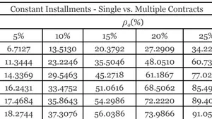
In Tables 8 to 13, a comparison of single and multiple contracts values of are presented. In terms of the annual cost of capital value , for different values of the monthly interest rate i, for contracts with term n ranging from 5 to 30 years.

Table 8: Fiscal Gain Comparison – monthly interest rate i=0.5% p.m.

Constant Installments - Single vs. Multiple Contracts
	$\rho_a(\%)$
n(years)	5%	10%	15%	20%	25%	30%
5	7.8844	15.9577	24.1931	32.5645	41.0469	49.6169
10	15.6432	32.6397	50.8269	70.0162	90.0068	110.5986
15	23.0441	49.2608	78.1367	109.0285	141.2650	174.2288
20	30.0078	65.3012	104.6218	146.4624	189.4352	232.4757
25	36.4748	80.3036	128.9813	179.8554	230.9162	280.9682
30	42.4060	93.9206	150.3444	207.9367	264.4861	319.0548

Table 9: Fiscal Gain Comparison – monthly interest rate i=1.0% p.m.

Constant Installments - Single vs. Multiple Contracts
	$\rho_a(\%)$
n(years)	5%	10%	15%	20%	25%	30%
5	7.4709	15.0921	22.8383	30.6852	38.6100	46.5914
10	14.0198	29.0432	44.9101	61.4475	78.4809	95.8444
15	19.5047	41.0777	64.2314	88.4350	113.1899	138.0765
20	23.9956	50.9828	79.8946	109.6788	139.5020	168.8095
25	27.6074	58.8032	91.7529	124.9283	157.3894	188.6977
30	30.4732	64.7578	100.2201	135.1035	168.6416	200.6545

Table 10: Fiscal Gain Comparison – monthly interest rate i=1.5% p.m.

Constant Installments - Single vs. Multiple Contracts
	$\rho_a(\%)$
n(years)	5%	10%	15%	20%	25%	30%
5	7.0804	14.2775	21.5676	28.9286	36.3396	43.7814
10	12.5912	25.9196	39.8353	54.1847	68.8199	83.6058
15	16.6379	34.6202	53.5221	72.9240	92.4622	111.8538
20	19.5387	40.7879	62.9157	85.2034	107.1470	128.4546
25	21.5953	44.9934	68.9223	92.4864	115.2285	136.9947
30	23.0520	47.7821	72.5546	96.4879	119.3078	141.0251

Table 11: Fiscal Gain Comparison – monthly interest rate i=2.0% p.m.

Constant Installments - Single vs. Multiple Contracts
	$\rho_a(\%)$
n(years)	5%	10%	15%	20%	25%	30%
5	6.7127	13.5130	20.3792	27.2909	34.2293	41.1772
10	11.3444	23.2246	35.5046	48.0510	60.7398	73.4620
15	14.3369	29.5463	45.2718	61.1867	77.0260	92.5980
20	16.2431	33.4752	51.0616	68.5062	85.4967	101.8767
25	17.4684	35.8643	54.2986	72.2220	89.4012	105.7919
30	18.2744	37.3076	56.0386	73.9866	91.0552	107.2993

Table 12: Fiscal Gain Comparison – monthly interest rate i=2.5% p.m.

Constant Installments - Single vs. Multiple Contracts
	$\rho_a(\%)$
n(years)	5%	10%	15%	20%	25%	30%
5	6.3673	12.7974	19.2702	25.7672	32.2715	38.7677
10	10.2616	20.9078	31.8173	42.8755	53.9793	65.0411
15	12.4920	25.5477	38.8727	52.2124	65.3724	78.2212
20	13.7799	28.1330	42.5733	56.7506	70.4649	83.6319
25	14.5535	29.5831	44.4504	58.8007	72.5100	85.5775
30	15.0423	30.4135	45.3891	59.6855	73.2758	86.2199

Table 13: Fiscal Gain Comparison – monthly interest rate i=3.0% p.m.

Constant Installments - Single vs. Multiple Contracts
	$\rho_a(\%)$
n(years)	5%	10%	15%	20%	25%	30%
5	6.0437	12.1289	18.2372	24.3519	30.4578	36.5415
10	9.3237	18.9184	28.6775	38.5028	48.3090	58.0256
15	11.0061	22.3717	33.8545	45.2545	56.4275	67.2821
20	11.9057	24.1377	36.3187	48.1948	59.6342	70.5915
25	12.4241	25.0787	37.4909	49.4210	60.8012	71.6479
30	12.7459	25.6036	38.0551	49.9222	61.2064	71.9629

{"image_source":{"path":"images/34686ba2795b5824810689f9d8f91c4d1e7617e7d2c4a44d4e19f2059782f4db.jpg"},"content":"","chart_caption":[{"type":"text","content":"Additionally, fixing the financing interest rate i, on 1% per month, Figures 1 and 2 depict the behavior of the fiscal gain, respectively for the cases where the opportunity cost varies from 5% to 30% per year, and when the length of the contract varies from 5 to 30 years."},{"type":"text","content":"Figure 1: Fiscal Gains x Opportunity Costs"}],"chart_footnote":[]} {"image_source":{"path":"images/801223cad21ffc23093a29e33ba563a186ad7eb9696ad1f6c91afad93e3f7516.jpg"},"content":"","chart_caption":[{"type":"text","content":"Figure 2: Fiscal Gains x Financial Terms"}],"chart_footnote":[]}

As shown, in all cases the fiscal gain is substantial. Which implies that the financial institution providing the loan should always choose the option of implementing multiple contracts.

5.2. The case of the "thirteenth wage"

Analogously, Tables 14 to 19 present the value of the fiscal gain , in terms of the annual value for different values of the monthly interest rate i, for contracts with length n of 5 to 30 years.

Additionally, fixing the financing interest rate i at 1% per month, Figures 3 and 4 depict the behavior of the fiscal gain, respectively for the cases where the opportunity cost varies from 5% to 30% per year, and when the length of the contract varies from 5 to 30 years, for the case of thirteen wages.

Table 14: Fiscal Gain Comparison 13 Wages – monthly interest rate i=0.5% p.m.

Constant Installments - Single vs. Multiple Contracts – 13 Wages
	$\rho_a(\%)$
n(years)	5%	10%	15%	20%	25%	30%
5	7.9499	16.0955	24.4096	32.8657	41.4385	50.1043
10	15.7020	32.7705	51.0423	70.3276	90.4246	111.1317
15	23.0986	49.3869	78.3498	109.3411	141.6869	174.7680
20	30.0583	65.4209	104.8252	146.7593	189.8330	232.9811
25	36.5212	80.4147	129.1682	180.1247	231.2740	281.4229
30	42.4484	94.0214	150.5109	208.1736	264.8009	319.4594

Table 15: Fiscal Gain Comparison 13 Wages – monthly interest rate i=1.0% p.m.

Constant Installments - Single vs. Multiple Contracts – 13Wages
	$\rho_a(\%)$
n(years)	5%	10%	15%	20%	25%	30%
5	7.5300	15.2162	23.0327	30.9551	38.9602	47.0264
10	14.0668	29.1469	45.0793	61.6900	78.8037	96.2536
15	19.5431	41.1647	64.3755	88.6429	113.4669	138.4274
20	24.0268	51.0542	80.0123	109.8471	139.7251	169.0926
25	27.6326	58.8604	91.8460	125.0606	157.5658	188.9256
30	30.4934	64.8031	100.2929	135.2076	168.7842	200.8451

Table 16: Fiscal Gain Comparison 13 Wages – monthly interest rate i=1.5% p.m.

Constant Installments - Single vs. Multiple Contracts – 13Wages
	$\rho_a(\%)$
n(years)	5%	10%	15%	20%	25%	30%
5	7.1337	14.3891	21.7423	29.1706	36.6531	44.1701
10	12.6290	26.0020	39.9688	54.3750	69.0718	83.9237
15	16.6652	34.6812	53.6218	73.0666	92.6515	112.0934
20	19.5585	40.8324	62.9884	85.3072	107.2857	128.6328
25	21.6098	45.0260	68.9755	92.5634	115.3343	137.1359
30	23.0629	47.8065	72.5949	96.5486	119.3953	141.1473

Table 17: Fiscal Gain Comparison 13 Wages – monthly interest rate i=2.0% p.m.

Constant Installments - Single vs. Multiple Contracts – 13Wages
	$\rho_a(\%)$
n(years)	5%	10%	15%	20%	25%	30%
5	6.7608	13.6135	20.5362	27.5082	34.5103	41.5252
10	11.3747	23.2906	35.6110	48.2020	60.9392	73.7132
15	14.3567	29.5902	45.3434	61.2890	77.1622	92.7714
20	16.2563	33.5050	51.1106	68.5772	85.5934	102.0036
25	17.4777	35.8855	54.3342	72.2754	89.4773	105.8967
30	18.2813	37.3235	56.0666	74.0310	91.1220	107.3949

Table 18: Fiscal Gain Comparison 13 Wages – monthly interest rate i=2.5% p.m.

Constant Installments - Single vs. Multiple Contracts – 13Wages
	$\rho_a(\%)$
n(years)	5%	10%	15%	20%	25%	30%
5	6.4107	12.8880	19.4115	25.9625	32.5239	39.0801
10	10.2863	20.9611	31.9032	42.9972	54.1399	65.2436
15	12.5068	25.5806	38.9265	52.2897	65.4762	78.3547
20	13.7894	28.1546	42.6095	56.8043	70.5398	83.7323
25	14.5601	29.5987	44.4775	58.8431	72.5723	85.6649
30	15.0473	30.4257	45.4117	59.7228	73.3331	86.3026

Table 19: Fiscal Gain Comparison 13 Wages – monthly interest rate i=3.0% p.m.

Constant Installments - Single vs. Multiple Contracts – 13Wages
	$\rho_a(\%)$
n(years)	5%	10%	15%	20%	25%	30%
5	6.0829	12.2107	18.3647	24.5279	30.6851	36.8226
10	9.3439	18.9622	28.7480	38.6028	48.4412	58.1926
15	11.0175	22.3974	33.8968	45.3161	56.5111	67.3909
20	11.9130	24.1546	36.3477	48.2389	59.6969	70.6771
25	12.4293	25.0912	37.5136	49.4576	60.8559	71.7255
30	12.7499	25.6139	38.0750	49.9557	61.2583	72.0381

{"image_source":{"path":"images/f7cb51ff095855654633d689ac1442a9e1389addcd9b460d522ed661fb24aadf.jpg"},"content":"","chart_caption":[],"chart_footnote":[]} {"image_source":{"path":"images/b1e6cd42ffedd155055713284adae5031114bdd12716b1edf2de8058ce8b082e.jpg"},"content":"","chart_caption":[{"type":"text","content":"Figure 3: Fiscal Gains x Opportunity Costs – 13 Wages"},{"type":"text","content":"Figure 4: Fiscal Gains x Financial Terms – 13 Wages"}],"chart_footnote":[]}

As shown, in all cases fiscal gain is very substantial. Therefore, given that implementing the policy of considering the "thirteenth wage" is beneficial to the borrower, the financial institution providing the loan, should also prefer to adopt the option of substituting a single contract by multiple contracts.

V. CONCLUSIONS

As shown in the other cases previously analyzed, cf. De-Losso et al. (2013), for the case of constant payments, de Faro (2021), for the case of periodic payments only, de Faro (2022), for the case of the constant amortization, de Faro and Lachtermacher (2023b), for the case of the an alternative version of the SACRE, and de Faro and Lachtermacher (2024), for the case of the German system of amortization, it always better for the financial institution providing the loan to implement the policy of multiple contracts.

Appendix A

\begin{array}{l} F = \frac {p \times \left\{1 - (1 + i) ^ {- n} \right\}}{i} + \frac {p \times \left\{1 - (1 + i _ {m}) ^ {- \ell} \right\}}{i _ {m}} \\F = p \times \left[ \frac {\left\{1 - (1 + i) ^ {- n} \right\}}{i} + \frac {\left\{1 - (1 + i _ {m}) ^ {- \ell} \right\}}{i _ {m}} \right] = p \times \left[ \frac {i _ {m} \left\{1 - (1 + i) ^ {- n} \right\} + i \left\{1 - (1 + i _ {m}) ^ {- \ell} \right\}}{i \times i _ {m}} \right] \\p = \frac {F \times i \times i _ {m}}{i _ {m} \left\{1 - (1 + i) ^ {- n} \right\} + i \left\{1 - (1 + i _ {m}) ^ {- \ell} \right\}} = \frac {F \times i \times i _ {m}}{i _ {m} \times \left\{1 - \frac {1}{(1 + i) ^ {n}} \right\} + i \times \left\{1 - \frac {1}{(1 + i _ {m}) ^ {\ell}} \right\}} \\p = \frac {F \times i \times i _ {m}}{i _ {m} \times \left\{\frac {(1 + i) ^ {n} - 1}{(1 + i) ^ {n}} \right\} + i \times \left\{\frac {(1 + i _ {m}) ^ {\ell} - 1}{(1 + i _ {m}) ^ {\ell}} \right\}} = \frac {F \times i \times i _ {m} \times (1 + i) ^ {n} \times (1 + i _ {m}) ^ {\ell}}{i _ {m} \times (1 + i _ {m}) ^ {\ell} \times [ (1 + i) ^ {n} - 1 ] + i \times (1 + i) ^ {n} [ (1 + i _ {m}) ^ {\ell} - 1 ]} \end{array}

since

\begin{array}{l} \left(1 + i\right) ^ {n} - 1 = \left(1 + i _ {m}\right) ^ {\ell} - 1 \Rightarrow \left(1 + i\right) ^ {n} = \left(1 + i _ {m}\right) ^ {\ell} \\p = \frac {F \times i \times i _ {m} \times (1 + i) ^ {n} \times (1 + i _ {m}) ^ {\ell}}{i _ {m} \times (1 + i _ {m}) ^ {\ell} \times [ (1 + i) ^ {n} - 1 ] + i \times (1 + i) ^ {n} [ (1 + i _ {m}) ^ {\ell} - 1 ]} = \frac {F \times i \times i _ {m} \times (1 + i) ^ {n}}{i _ {m} \times [ (1 + i) ^ {n} - 1 ] + i \times [ (1 + i _ {m}) ^ {\ell} - 1 ]} \\p = \frac {F \times i \times i _ {m} \times (1 + i) ^ {n}}{i _ {m} \times [ (1 + i) ^ {n} - 1 ] + i \times [ (1 + i) ^ {n} - 1 ]} = \frac {F \times i \times i _ {m} \times (1 + i) ^ {n}}{[ (1 + i) ^ {n} - 1 ] \times (i + i _ {m})} \end{array}

− Conflict of Interest

The authors declare no conflict of interest.

− Ethical Approval

Not applicable

− Data Availability

The datasets used in this study are openly available at [repository link] and the source code is available on GitHub at [GitHub link].

− Funding

This work did not receive any external funding.

− References

7 Cites in Article

REFERENCE FORMAT

− Cite this article

Generating citation...

Classification
1

JEL Code: G21
Version of record

v1.0
Issue date

21 February 2025
Language

en

Download Article Access OJS

Open Access

Research Article

CC-BY-NC 4.0

LJRMB Volume 25 LJRMB Volume 25 Issue 1, Pg. 69-81

Explore Journal

Read LJRMB Volume 25 Issue 1 Explore LJRMB Volume 25

Views 2.8K

Downloads 111

Year

Special Issue

Launch a focused special issue to highlight research, emerging trends, and expert insights in your academic field.

Multiple Contracts: The Case of Periodic Balloon Payments – Constant Installments

IntelliPaper

− Abstract

− Explore Digital Article Text

I. INTRODUCTION

II. THE CASE OF A SINGLE CONTRACT

III. THE CASE OF MULTIPLE CONTRACTS

4.1. Reduction in the value of the installments

5.1. The case of periodic payments only

5.2. The case of the "thirteenth wage"

V. CONCLUSIONS

Appendix A

− Conflict of Interest

− Ethical Approval

− Data Availability

− Funding

− References

− Cite this article

Classification

Version of record

Issue date

Language

Special Issue

Next Research

Copy of Cardiovascular Risk Factors and Cardiovascular Risk in People Living with HIV: Comparison of Four Cardiovascular Risk Prediction Algorithms

Privacy preferences

Multiple Contracts: The Case of Periodic Balloon Payments – Constant Installments

IntelliPaper

Request Review Access

Order Article Reprints

− Abstract

− Explore Digital Article Text

I. INTRODUCTION

II. THE CASE OF A SINGLE CONTRACT

III. THE CASE OF MULTIPLE CONTRACTS

4.1. Reduction in the value of the installments

5.1. The case of periodic payments only

5.2. The case of the "thirteenth wage"

V. CONCLUSIONS

Appendix A

− Conflict of Interest

− Ethical Approval

− Data Availability

− Funding

− References

− Cite this article

− Related Research

Classification

Version of record

Issue date

Language

Special Issue

Next Research

Copy of Cardiovascular Risk Factors and Cardiovascular Risk in People Living with HIV: Comparison of Four Cardiovascular Risk Prediction Algorithms

Privacy preferences