Optimizing Self-Insurance

The project manager(s) will want to avoid incurring excess costs, due to damages/losses that could have been insured (In this regard, the lower the liability retained, the more protection will be provided for the project, ceteris paribus).

The project manager(s) will want to avoid passing on too much money to insurers in the form of premiums, if there is a way to demonstrate that such premiums are unnecessary or redundant (In this regard, the higher the liability retained, the more savings will be obtained with respect to premium payments, ceteris paribus).

The risk manager(s) responsible for the project will aim for an optimum retention level such that the sum of premiums paid and losses incurred (i.e. the total outgo with respect to insurance) is minimized.

I. THE MATHEMATICS

1.1 Selecting an Appropriate Premium Principle

Optimizing the retention level requires the application of one of the premium principles from actuarial science.

For purposes of illustration, this article will utilize the Exponential Premium Principle, an authoritatively recognized method of premium formulation (1) which will be applied in two steps as follows:

Step 1: Premium Payable

Here:

a represents a non-negative scalar, which provides a numerical scale for risk-aversion

S represents the (random) total liability payable for insurable events over the coverage period

R represents a retention limit determined by the project risk manager

& represents the expected value function for the liability above To further concretize the illustration, it will be assumed that all the above formula parameters are explicitly known:

■ a: 0.05

■ S: A gamma distribution with shape parameter 0.7 and scale parameter 7.5

■ R: 4.99 units

• Here the expression 'units' is employed, to avoid being locked into any specific currency or denomination

■ So for example, a unit could be 10 million US dollars or 1 billion Japanese yen

The formula for the premium principle can then be applied by the systematic steps below.

1.2 First, Assuming Losses Follow the Above Gamma Distribution

Here 'losses' refers to payments from the project, due solely to peril/risk incurred in the normal course of operations.

GD = GammaDistribution[0.7, 7.5]

Graph of the Cumulative Distribution Function of Losses {"image_source":{"path":"images/54c59abd3cebf09b6219adf724a53f1966cc0937a69cef56479d87e2d6bc24d5.jpg"},"content":"","chart_caption":[],"chart_footnote":[]}

Next, Obtain a Computational Proxy For (The Upper Limit of The Distribution Function)

U = InverseCDF[GD, 0.999999999]

This produces a value of 146.669.

1.3 Then Apply the Premium Principle In Practical Terms

If we denote the cumulative distribution function of S at a value Y as CDF[S, Y], and the corresponding probability density function as PDF[S, Y], then we will have (2):

Applying our chosen premium principle to the specific values defined above, we determine the premium, P, to be:

The result is 3.25533 units.

Step 2: Insurer Limits

We will now consider the situation where the insurer contractually imposes a limit, L, on the amount of liability for which it is responsible. In such a situation, the insurer will pay claims up to L, and will disregard claim amounts greater than L. This will necessarily reduce the premium payable by the project. Application of the Exponential Premium Principle will yield:

If we keep the same risk-aversion parameter, loss distribution function and retention as previously used, but also impose a limit of 25 units, we would obtain the following premium, P:

P = Prem[0.05, GD, 4.99, 25]

The result is 1.87142 units.

II. SOLVING THE RETENTION PROBLEM

The way to obtain the solution for optimum retention then becomes clear:

Derive a function of R (keeping all other parameters at the constant levels above) based on the premium principle, and solve for the value of R that minimizes the function.

In short, minimize:

III. THE FINAL RESULT

The practical approach to obtaining the desired result, consists of:

■ (a) defining a comprehensive range of possible values of R

■ (b) calculating the corresponding values of

■ (c) graphing the results (d) identifying the minimum value from observation of the graph

The illustrative example used in this paper proceeds as follows:

■ Range of possible value of R: 5.00 to 9.99

■ Incremental step in values of R: 0.01

3.1 Observation of Graph

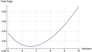
The results are graphed below. Observation shows the required minimum to be between 6.5 and 7 units.

{"image_source":{"path":"images/b0d70526566e33d7fcfa01a6fa16da4020895f6e71675e8ee2efdf1dbd3e48e8.jpg"},"content":"","chart_caption":[],"chart_footnote":[]} By applying appropriate numerical techniques to refine/improve the precision of the model, it can be shown that the correct answer is between 6.59 and 6.6 units.

VI. ANALYSIS

The above treatise is for illustration only.

Practical application in a real setting would require intensive statistical research to arrive at the distribution function that best fits the insurable losses. Similarly, investigation and study would be required to determine the best representative risk-aversion parameter.

Note however, that even if precise definitions of these parameters cannot be obtained, the project risk manager(s) could still provide useful information by applying the model in a simulation setting, with multiple runs to show results under various 'what if' situations and combinations of situations.

The approach outlined in this article could therefore, at the very least, form a foundation for addressing the important issue of self-insuring projects.

Lloyd Foster FSA MAAA

APPENDIX

Derivation of Premium Formula When Insurer Limit, £, is Imposed When There Are No Limits

It is instructive to first see how the formula is derived when there are no limits. The relevant point is that the insurer liability between 0 and R is identically 0. We therefore take this fact into account when applying the premium principle.

Successively:

When Limit, , is Imposed In the case of a limit, L, we note that in addition to the above restriction, the insurer liability between R and U is identically 0. Again, we take this fact into account when applying the premium principle.

First, let

Then successively:

1. An Introduction to Mathematical Risk Theory, Chapter 5, Pages 67 and 68, by Hans U Gerber

2. An Introduction to Mathematical Risk Theory, Chapter 7, Pages 96 and 97, by Hans U Gerber