Quantization of Dark Energy Particles and Sarkar Limit

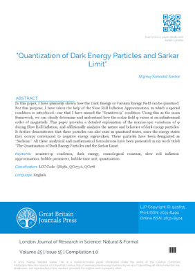
In this paper, I have primarily shown how the Dark Energy or Vacuum Energy Field can be quantized. For this purpose, I have taken the help of the Slow Roll Inflation Approximation, in which a special condition is introduced—one that I have named the “Sensitive-φ” condition. Using this as the main framework, we can clearly determine and understand how the scalar field φ varies at an infinitesimal order of magnitude. This paper provides a detailed explanation of the microscopic variations of φ during Slow Roll Inflation, and additionally analyzes the nature and behavior of dark energy particles. It further demonstrates that these particles can also exist in quantized states, since the energy states they occupy correspond to negative energy eigenvalues. These particles have been designated as “Sarkons.” All these analytical and mathematical formulations have been presented in my work titled “The Quantization of Dark Energy Particles and the Sarkar Limit.”