I. INTRODUCTION
Let ( ) be complex-valued continuous functions on the interval . Consider the system
\[t ≥ t_0, \left\{
\begin{array}{l}
\phi^{\prime}(t) = a_{1 1}(t) \phi(t) + a_{1 2}(t) \boldsymbol{\psi}(t); \\
\boldsymbol{\psi}^{\prime}(t) = a_{2 1}(t) \phi(t) + a_{2 2}(t) \boldsymbol{\psi}(t),
\end{array}
\right.
\tag{1.1}\]
. Study of the question of stability of solutions of differential equations and systems of differential equations, in particular of system (1.1), is an important problem of qualitative theory of differential equations and many works are devoted to it (see [1], [2] and cited works therein [3 - 10]). The fundamental theorem of R. Bellman (see [2], pp. 168, 169) reduces the study of boundedness of solutions of wide class of nonlinear systems to the study of stability of linear systems of differential equations. Many problems of mechanics, physics and other natural sciences are connected with the study of stability of the linear systems of differential equations (in particular of the linear differential equations) too (see for example ). One of ways to study the mentioned above question is the use of different methods of estimations of solutions of systems of being studied equations (see ).
In this paper some estimates of solutions of the system in terms of its coefficients are obtained. To obtain them it was used the method of approximation of solutions of by solutions of system with piecewise constant coefficients (the discrete ordinates method).
\[\text {Denote:} P (t) \equiv a _ {1 2} (t) \exp \Bigl \{\int_ {t _ {0}} ^ {t} \bigl [ a _ {2 2} (\tau) - a _ {1 1} (\tau) \bigr ] d \tau \Bigr \}, Q (t) \equiv a _ {2 1} (t) \exp \Bigl \{\int_ {t _ {0}} ^ {t} \bigl [ a _ {1 1} (\tau) - a _ {2 2} (\tau) \bigr ] d \tau \Bigr \}\]
. In this article we will study the following two principal cases:
\[\begin{array}{l l} A) P (t) > 0, & Q (t) < 0, \quad t \geq t _ {0}; \\B) P (t) > 0, & Q (t) > 0, \quad t \geq t _ {0} \end{array}\]
(the case , , , is similar to the case A), and the case , , , is reducible to the case B) by the simple substitution . The case A) can be geometrically interpreted as a case, when the origin of coordinates of phase plane of variables u, v is a "center" or a "focus" and the case B) as a "saddle" with respect to the curves , , where are the solutions of the system
\[\left\{
\begin{array}{l}
u ^ {\prime} (t) = P (t) v (t); \\
v ^ {\prime} (t) = Q (t) u (t)
\end{array}
\right.\tag{1.2}\]
. On examples the obtained results are compared with the results obtained by methods of Liapunov, Yu. S. Bogdanov, T. Wazevski, estimates of solutions by logarithmic norm of S. M. Lozinski and of freezing.
II. AUXILIARY PROPOSITIONS
Lemma 2.1. For each solution of the system (1.1) and for each and there exists piecewise constant functions , , , such, that the solutions of the system
\[\left\{
\begin{array}{l}
\phi^{\prime}(t) = \widetilde{a}_{11}(t) \phi(t) + \widetilde{a}_{12}(t) \boldsymbol{\psi}(t); \\
\psi^{\prime}(t) = \widetilde{a}_{21}(t) \phi(t) + \widetilde{a}_{22}(t) \boldsymbol{\psi}(t),
\end{array}
\right.
\tag{2.0}\]
. with , satisfy the inequalities: , .
The proof of this lemma is not difficult, and we omit it.
Remark 2.1. By a solution of the system (2.0) we will mean a pair of absolutely continuous functions and , satisfying (2.0) almost everywhere on .
Let be a finite or infinite sequens, and let , , , . Consider the Cauchy problem
\[\left\{
\begin{array}{l}
u ^ {\prime} (t) = \widetilde {p} (t) v (t); \\
v ^ {\prime} (t) = - \widetilde {q} (t) u (t); \\
u (t _ {0}) = u _ 0, v (t _ {0}) = v _ 0
\end{array}
\right.
\tag{2.1}\]
. Any solution of this system we will seek in the form
\[u (t) = A _ {j} \sin (\sqrt {l _ {j}} t + \omega_ {j}), \quad v (t) = A _ {j} \sqrt {h _ {j}} \cos (\sqrt {l _ {j}} t + \omega_ {j}), \quad t \in [ t _ {j}, t _ {j + 1}),\tag{2.2}\]
where , and , are the sought constants, . By virtue of initial conditions of problem (2.1) the unknowns and we determine by solving the system
\[\left\{ \begin{array}{l l} A _ {0} \sin \big (\sqrt {l _ {0}} t _ {0} + \omega_ {0} \big) = u _ {(0)}; \\A _ {0} \sqrt {h _ {0}} \cos \big (\sqrt {l _ {0}} t _ {0} + \omega_ {0} \big) = v _ {(0)}, \end{array} \right.
\tag{2.3}\]
and the remaining unknowns by successive solving of the systems
\[\left\{ \begin{array}{l} A _ {j + 1} \sin \bigl (\sqrt {l _ {j + 1}} t _ {j + 1} + \omega_ {j + 1} \bigr) = A _ {j} \sin \bigl (\sqrt {l _ {j}} t _ {j + 1} + \omega_ {j} \bigr); \\ A _ {j + 1} \sqrt {h _ {j + 1}} \cos \bigl (\sqrt {l _ {j + 1}} t _ {j + 1} + \omega_ {j + 1} \bigr) = A _ {j} \sqrt {h _ {j}} \cos \bigl (\sqrt {l _ {j}} t _ {j + 1} + \omega_ {j} \bigr), \end{array} \right.\tag{2.4}\]
. From (2.3) it follows
\[A_{0} = u^{2}_{(0)} + \frac{v^{2}_{(0)}}{h_{0}}.\]
Denote: , , . From (2.4) it is easy to derive the equalities:
\[A _ {j + 1} ^ {2} = A _ {j} ^ {2} \left[ \frac {h _ {j} + h _ {j + 1}}{2 h _ {j + 1}} + \frac {h _ {j} - h _ {j + 1}}{2 h _ {j + 1}} \cos 2 \alpha_ {j} \right], \quad A _ {j} ^ {2} = A _ {j + 1} ^ {2} \left[ \frac {h _ {j} + h _ {j + 1}}{2 h _ {j}} + \frac {h _ {j + 1} - h _ {j}}{2 h _ {j}} \cos 2 \beta_ {j} \right],\]
From here it follows
\[|A_{j+1}| \leq |A_j| \leq \sqrt{\frac{h_{j+1}}{h_j}} |A_{j+1}| \quad for \quad h_j \leq h_{j+1};\]
\[|A_{j}| \leq |A_{j+1}| \leq \sqrt{\frac{h_{j}}{h_{j+1}}} |A_{j}| \quad for \quad h_{j} \geq h_{j+1};\]
From (2.2) it follows:
\[u ^ {2} (t) \frac {1}{h _ {j}} + v ^ {2} (t) = A _ {j} ^ {2}, t \in [ t _ {j}, t _ {j + 1}), j = 0, 1, 2, \dots .\tag{2.8}\]
Let the initial values and be real. Then and will be real valued. Therefore, from (2.8) we will have:
\[\min \{1, h _ {j} ^ {1} \} A _ {j} ^ {2} \leq u ^ {2} (t) + v ^ {2} (t) \leq \max \{1, h _ {j} ^ {1} \} A _ {j} ^ {2}, t \in [ t _ {j}, t _ {j + 1}),\tag{2.9}\]
where .
Definition 2.1. We shall say, that a continuous on the interval function belongs to the class , if there exists an infinitely large sequence such, that is a nondecreasing on the interval and nonincreasing on the interval function, . The numbers , we shall call points of possible extremums of the function .
Let , and let , be the points of possible extremums of . Note, that if , , then is a nondecreasing function and if , , then is a nonincreasing function. Let , . Consider the functions
\[r_{S}^{-}(t) \equiv \left\{ \begin{array}{l l} 1, & t \in [\xi_0;\xi_1]; \\ \sqrt{\frac{S(\xi_1)}{S(t)}}, & t \in [\xi_1;\xi_2]; \\ \prod_{k=1}^{n} \sqrt{\frac{S(\xi_{2k-1})}{S(\xi_{2k})}}, & t \in [\xi_{2n};\xi_{2n+1}], \, n = 1,2,...; \\ \left[ \prod_{k=1}^{n-1} \sqrt{\frac{S(\xi_{2k-1})}{S(\xi_{2k})}} \right] \sqrt{\frac{S(\xi_{2n-1})}{S(t)}}, & t \in [\xi_{2n-1};\xi_{2n}], \, n = 2,3,... \end{array} \right.\]
\[r_{S}^{+}(t) \equiv \left\{
\begin{array}{l l}
\sqrt{\frac{S(t)}{S(\xi_0)}}, & t \in [\xi_0; \xi_1]; \\
\prod_{k = 0}^n \sqrt{\frac{S(\xi_{2k+1})}{S(\xi_{2k})}}, & t \in [\xi_{2n+1}; \xi_{2n+2}], \, n = 0, 1,...; \\
\left[ \prod_{k = 9}^{n-1} \sqrt{\frac{S(\xi_{2k-1})}{S(\xi_{2k})}} \right] \sqrt{\frac{S(t)}{S(\xi_{2n})}}, & t \in [\xi_{2n}; \xi_{2n+1}], \, n = 1, 2,...
\end{array}
\right.\]
Let be absolutely continuous. Then ,
\[\sqrt{\frac{S(\xi_{2k-1})}{S(\xi_{2k})}} = \exp\left\{-\frac{1}{2} \int_{\xi_{2k-1}}^{\xi_{2k}} \frac{S'(\tau)}{S(\tau)} d\tau\right\}, k = 1, 2, \ldots\]
\[r_{S}^{-}(t) = \exp\left\{\frac{1}{2}\int_{t_0}^{t}\frac{S_{(-)}'(\tau)}{S(\tau)}d\tau\right\},\quad t \geq t_0,\]
where . By analogy it shows, that
\[r_{S}^{+}(t) = \exp\left\{\frac{1}{2}\int_{t_0}^{t}\frac{S_{(+)}'(\tau)}{S(\tau)}d\tau\right\},\quad t \geq t_0,\]
where . It is clear that , in all the points of existence of . From here, from (2.10) and (2.11) it follows:
\[r_{S}^{-}(t) = \sqrt[4]{\frac{S(t_{0})}{S(t)}} \exp\left\{\frac{1}{4} \int_{t_{0}}^{t} \frac{|S'(\tau)|}{S(\tau)} d\tau\right\}, \quad t \geq t_{0},\]
\[r_{S}^{+}(t) = \sqrt[4]{\frac{S(t)}{S(t_{0})}} \exp\left\{\frac{1}{4} \int_{t_{0}}^{t} \frac{|S'(\tau)|}{S(\tau)} d\tau\right\}, \quad t \geq t_{0},\]
Let and be positive and continuous functions on the interval . Consider the system of equations
\[\left\{
\begin{array}{l}
u ^ {\prime} (t) = p (t) v (t); \\
v ^ {\prime} (t) = - q (t) u (t)
\end{array}
\right.
\tag{2.14}\]
. Let us introduce some notations, necessary in the sequel: , , , , , where and are continu- ous functions on the interval , is a absolutely continuous and positive function on the interval with locally finite variation.
Lemma 2.2. Let be an absolutely continuous function with locally finite variation. Then for every solution of the system (2.14) the following inequalities hold:
\[\frac {g (t _ {0}) g (t)}{r _ {h} (t)} | | (u (t _ {0}), v (t _ {0}) | | \leq | | (u (t), v (t)) | | \leq G (t _ {0}) G (t) | | (u (t _ {0}), v (t _ {0})) | | r _ {h} (t),\tag{2.15}\]
\[t \geq t _ {0}\]
Proof. Let us consider first the case, when has the additional property: . Let be a nontrivial real valued solution of the system (2.14), and let be the possible extremums of the function . Let and be fixed. By virtue of Lemma 2.1 there exist piecewise constant functions and such, that the solution of the system
\[\left\{
\begin{array}{l}
u ^ {\prime} (t) = \widetilde {\widetilde {p}} (t) v (t); \\
v ^ {\prime} (t) = - \widetilde {\widetilde {q}} (t) u (t)
\end{array}
\right.\]
, with , satisfies the inequalities:
\[| \widetilde {u} (t _ {1}) - u _ {0} (t _ {1}) | \leq \varepsilon , \quad | \widetilde {v} (t _ {1}) - v _ {0} (t _ {1}) | \leq \varepsilon .\tag{2.16}\]
Without loss of generality we will assume that , , , , ; , , ; the function is nondecreasing on the intervals and nonincreasing on the intervals , . Then by (2.5) - (2.7), (2.9) the following inequalities hold
\[g_1(t_0)g_1(t_1)\|(u_0(t_0),v_0(t_0))\|\sqrt{\frac{h(\xi_0)}{h(t_1)}} \leq \|(\widetilde{u}(t_1),\widetilde{v}(t_1))\| \leq G_1(t_0)G_1(t_1)\|(u_0(t_0),v_0(t_0))\|,\]
\[\mathrm{if} t _ {1} \in [ \xi_ {0}, \xi_ {1} ];\]
\[g _ {1} (t _ {0}) g _ {1} (t _ {1}) | | (u _ {0} (t _ {0}), v _ {0} (t _ {0})) | | \sqrt {\frac {h (\xi_ {0})}{h (t _ {1})}} \leq | | (\widetilde {u} (t _ {1}), \widetilde {v} (t _ {1})) | | \leq\]
\[\leq G _ {1} (t _ {0}) G _ {1} (t _ {1}) | | (u _ {0} (t _ {0}), v _ {0} (t _ {0})) | | \sqrt{\frac{h (\xi_ {1})}{h (t _ {1})}}, if t _ {1} \in [ \xi_ {1}, \xi_ {2} ];\]
\[g_{1}(t_{0})g_{1}(t_{1})\|(u_{0}(t_{0}),v_{0}(t_{0}))\|\left[\prod_{k=0}^{n}\sqrt{\frac{h(\xi_{2k})}{h(\xi_{2k+1})}}\right]\sqrt{\frac{h(\xi_{2n})}{h(t_{1})}}\leq\|\!(\widetilde{u}(t_{1}),\widetilde{v}(t_{1}))\|\leq\]
\[\leq G _ {1} (t _ {0}) G _ {1} (t _ {1}) | | (u _ {0} (t _ {0}), v _ {0} (t _ {0})) | | \prod_ {k = 1} ^ {n} \sqrt{\frac{h (\xi_ {2 k - 1})}{h (\xi_ {2 k})}}, if t _ {1} \in [ \xi_ {2 n}, \xi_ {2 n + 1} ], n = 1, 2, \dots ;\]
\[g_{1}(t_{0})g_{1}(t_{1})\|(u_{0}(t_{0}),v_{0}(t_{0}))\|\prod_{k=0}^{n}\sqrt{\frac{h(\xi_{2k})}{h(\xi_{2k+1})}}\leq\|(\widetilde{u}(t_{1}),\widetilde{v}(t_{1}))\|\leq\]
\[\leq G _ {1} (t _ {0}) G _ {1} (t _ {1}) | | (u _ {0} (t _ {0}), v _ {0} (t _ {0})) | | \left[ \prod_ {k = 0} ^ {n - 1}, \sqrt{\frac{h (\xi_ {2 k + 1})}{h (\xi_ {2 k + 2})}} \right] \sqrt{\frac{h (\xi_ {2 n + 1})}{h (t _ {1})}}, if t _ {1} \in [ \xi_ {2 n + 1}, \xi_ {2 n + 2} ],\]
, where , , . It follows from here, that
\[\frac{g_{1}(t_{0}) g_{1}(t_{1}) \|(u_{0}(t_{0}), v_{0}(t_{0}))\|}{r_{h}^{+}(t_{1})} \leq \|(\widetilde{u}(t_{1}), \widetilde{v}(t_{1}))\| \leq G_{1}(t_{0})G_{1}(t_{1}) \|(u_{0}(t_{0}), v_{0}(t_{0}))\| r_{h}^{-}(t_{1}).\]
By analogy (making the substitution , interchanging and , as well as interchanging and ) we come to the inequalities
\[\frac {g _ {2} (t _ {0}) g _ {2} (t _ {1}) | | (u _ {0} (t _ {0}) , v _ {0} (t _ {0})) | |}{r _ {h _ {1}} ^ {+} (t _ {1})} \leq | | (\widetilde {u} (t _ {1}), \widetilde {v} (t _ {1})) | | \leq\]
\[\leq G_{2}(t_{0})G_{2}(t_{1})||(u_{0}(t_{0}),v_{0}(t_{0}))||r_{h_{1}}^{-}(t_{1}),\]
where , , . From here and from (2.17) we obtain:
\[\sqrt {\frac {g _ {1} (t _ {0}) g _ {1} (t _ {1}) g _ {2} (t _ {0}) g _ {2} (t _ {1})}{r _ {h} ^ {+} (t _ {1}) r _ {h _ {1}} ^ {+} (t _ {1})}} | | (u _ {0} (t _ {0}), v _ {0} (t _ {0})) | | \leq | | (\widetilde {u} (t _ {1}), \widetilde {v} (t _ {1}) | | \leq\]
\[\leq \sqrt{G_{1}(t_{0}) G_{1}(t_{1}) G_{2}(t_{0}) G_{2}(t_{1})} \| (u_{0}(t_{0}), v_{0}(t_{0})) \| \sqrt{r_{h}^{-}(t_{1}) r_{h_{1}}^{-}(t_{1})}.\]
Obviously,
\[g _ {1} (t) g _ {2} (t) = g ^ {2} (t), G _ {1} (t) G _ {2} (t) = G ^ {2} (t), \quad t \geq t _ {0}.\tag{2.19}\]
Note (due to (2.12) and (2.13)), that , . Then . From here, from (2.18) and (2.19) we obtain:
\[\frac {g (t _ {0}) g (t _ {1}) | | (u _ {0} (t _ {0}) , v _ {0} (t _ {0})) | |}{r _ {h} (t _ {1})} \leq | | (\widetilde {u} (t _ {1}), \widetilde {v} (t _ {1}) | | \leq\]
\[\leq G(t_{0})G(t_{1})||(u_{0}(t_{0}),v_{0}(t_{0}))||r_{h}(t_{1}).\]
From here and from (2.16) it follows:
\[\frac{g(t_{0}) g(t_{1}) \|(u_{0}(t_{0}), v_{0}(t_{0}))\|}{r_{h}(t_{1})} - \sqrt{2} \varepsilon \leq \|(u_{0}(t_{1}), v_{0}(t_{1}))\| \leq\]
\[\leq G(t_{0})G(t_{1})\|(u_{0}(t_{0}), v_{0}(t_{0}))\| r_{h}(t_{1}) + \sqrt{2} \varepsilon.\]
By the arbitrariness of from here we will have:
\[\frac {g (t _ {0}) g (t _ {1}) | | (u _ {0} (t _ {0}) , v _ {0} (t _ {0})) | |}{r _ {h} (t _ {1})} \leq | | (u _ {0} (t _ {1}), v _ {0} (t _ {1}) | | \leq\]
\[\leq G(t_{0})G(t_{1})||(u_{0}(t_{0}),v_{0}(t_{0}))||r_{h}(t_{1}).\]
Let be an arbitrary (complex) solution of the system (2.14). Since , where , are some real solutions of the system (2.14), by (2.20) we will get:
\[\left[ \frac {g (t _ {0}) g (t _ {1})}{r _ {h} (t _ {1})} \right] ^ {2} \sum_ {j = 1} ^ {2} | | (u _ {j} (t _ {0}), v _ {j} (t _ {0})) | | ^ {2} \leq \sum_ {j = 1} ^ {2} | | (u _ {j} (t _ {1}), v _ {j} (t _ {1})) | | ^ {2} \leq\]
\[\leq \left[ G(t_0)G(t_1)r_h(t_1) \right]^2 \sum_{j=1}^2 \| (u_j(t_0), v_j(t_0)) \|^2.\]
Taking into account the equality , from here we will have:
\[\frac {g (t _ {0}) g (t _ {1}) | | (u (t _ {0}) , v (t _ {0})) | |}{r _ {h} (t _ {1})} \leq | | (u (t _ {1}), v (t _ {1}) | | \leq G (t _ {0}) G (t _ {1}) | | (u (t _ {0}), v (t _ {0})) | | r _ {h} (t _ {1}).\]
By virtue of arbitrariness of from here it follows (2.15). Thus, we have proved (2.15) under the additional assumption . Let us prove it in the general case. Let be the space of absolutely continuous functions of finite variation on the interval with the norm . Obviously the set of rational functions is everywhere dense in . In view of this we choose polynomials and such, that , , , and such, that for each fixed and the following inequalities hold
\[\left| \frac{g (t _ {0}) g (t _ {1})}{r _ {h} (t _ {1})} - \frac{\widetilde{g} (t _ {0}) \widetilde{g} (t _ {1})}{r _ {\widetilde{h}} (t _ {1})} \right| \leq \varepsilon , \left| G (t _ {0}) G (t _ {1}) r _ {h} (t _ {1}) - \widetilde{G} (t _ {0}) \widetilde{G} (t _ {1}) r _ {\widetilde{h}} (t _ {1}) \right| \leq \varepsilon ,\]
\[where \widetilde{g}(t) \equiv \min\left\{\sqrt[4]{\widetilde{h}(t)}, \sqrt[4]{\widetilde{h}_1(t)}\right\}, \widetilde{G}(t) \equiv \max\left\{\sqrt[4]{\widetilde{h}(t)}, \sqrt[4]{\widetilde{h}_1(t)}\right\}, \widetilde{h}(t) \equiv \frac{q_1(t)}{p_1(t)},\]
, as well as (by Lemma 2.1) the following inequalities hold
\[\left| u \left(t _ {1}\right) - \widetilde {u} \left(t _ {1}\right) \right| \leq \varepsilon , \quad \left| v \left(t _ {1}\right) - \widetilde {v} \left(t _ {1}\right) \right| \leq \varepsilon ,\tag{2.22}\]
where is the solution of the system
\[\left\{
\begin{array}{l}
u ^ {\prime} (t) = p _ {1} (t) v (t); \\
v ^ {\prime} (t) = q _ {1} (t) u (t)
\end{array}
\right.\]
, with , . Since obviously , by already proven
\[\frac{\widetilde{g}(t_0)\widetilde{g}(t_1)\|(u(t_0),v(t_0))\|}{r_{\widetilde{h}}(t_1)} \leq \| (\widetilde{u}(t_1),\widetilde{v}(t_1)) \| \leq \widetilde{G}(t_0)\widetilde{G}(t_1)\|(u(t_0),v(t_0))\| r_{\widetilde{h}}(t_1).\]
From here, from (2.21) and (2.22) it follows
\[\frac {g (t _ {0}) g (t _ {1}) | | (u (t _ {0}) , v (t _ {0})) | |}{r _ {h} (t _ {1})} - [ \sqrt {2} + | | (u (t _ {0}), v (t _ {0})) | | ] \varepsilon \leq | | (u (t _ {1}), v (t _ {1}) | | \leq\]
\[\leq G (t _ {0}) G (t _ {1}) | | (u (t _ {0}), v (t _ {0})) | | r _ {h} (t _ {1}) + [ \sqrt {2} + | | (u (t _ {0}), v (t _ {0})) | | ] \varepsilon .\]
By virtue of arbitrariness of , and from here it follows (2.15). The lemma is proved.
Let us consider the Cauchy problem
\[\left\{
\begin{array}{l}
u ^ {\prime} (t) = \widetilde {p} (t) v (t); \\
v ^ {\prime} (t) = \widetilde {q} (t) u (t); \\
u (t _ {0}) = u _ 0, v (t _ {0}) = v _ 0
\end{array}
\right.
\tag{2.23}\]
. Its solution we will seek in the form
\[\left\{ \begin{array}{l l} u (t) = A _ {j} \sqrt {p _ {j}} \exp \{\sqrt {l _ {j}} t \} + B _ {j} \sqrt {p _ {j}} \exp \{- \sqrt {l _ {j}} t \}; \\ v (t) = A _ {j} \sqrt {q _ {j}} \exp \{\sqrt {l _ {j}} t \} - B _ {j} \sqrt {q _ {j}} \exp \{- \sqrt {l _ {j}} t \}, \end{array} \right.
\tag{2.24}\]
. The unknowns and we can find by solving the system
\[\left\{ \begin{array}{l} A _ {0} \sqrt {p _ {0}} \exp \{\sqrt {l _ {0}} t _ {0} \} + B _ {0} \sqrt {p _ {0}} \exp \{- \sqrt {l _ {0}} t _ {0} \} = u _ {(0)}; \\A _ {0} \sqrt {q _ {0}} \exp \{\sqrt {l _ {0}} t _ {0} \} - B _ {0} \sqrt {q _ {0}} \exp \{- \sqrt {l _ {0}} t _ {0} \} = v _ {(0)}, \end{array} \right.\tag{2.25}\]
and the remaining unknowns we can find by successive solving the systems
\[\left\{ \begin{array}{l l} A _ {j} \sqrt {p _ {j}} \exp \{\sqrt {l _ {j}} t _ {j} \} + B _ {j} \sqrt {p _ {j}} \exp \{- \sqrt {l _ {j}} t _ {j} \} = u (t _ {j}); \\ A _ {j} \sqrt {q _ {j}} \exp \{\sqrt {l _ {j}} t _ {j} \} - B _ {j} \sqrt {q _ {j}} \exp \{- \sqrt {l _ {j}} t _ {j} \} = v (t _ {j}) \end{array} \right.\]
We have:
\[A _ {j} = \frac {u (t _ {j}) \sqrt {q _ {j}} + v (t _ {j}) \sqrt {p _ {j}}}{2 \sqrt {l _ {j}}} \exp \{- \sqrt {l _ {j}} t _ {j} \}, B _ {j} = \frac {u (t _ {j}) \sqrt {q _ {j}} - v (t _ {j}) \sqrt {p _ {j}}}{2 \sqrt {l _ {j}}} \exp \{- \sqrt {l _ {j}} t _ {j} \}.\]
From here, from (2.24) and (2.25) it follows
\[\left\{ \begin{array}{l} u (t) = u (t _ {j}) \operatorname{ch} \{\sqrt {l _ {j}} (t - t _ {j}) \} + v (t _ {j}) \sqrt {\frac {p _ {j}}{q _ {j}}} \operatorname{sh} \{\sqrt {l _ {j}} (t - t _ {j}) \}; \\v (t) = v (t _ {j}) \operatorname{ch} \{\sqrt {l _ {j}} (t - t _ {j}) \} + u (t _ {j}) \sqrt {\frac {q _ {j}}{p _ {j}}} \operatorname{sh} \{\sqrt {l _ {j}} (t - t _ {j}) \}, \end{array} \right.
\tag{2.26}\]
From here it is easy to derive the equalities
\[\sqrt {q _ {j}} u (t) + \sqrt {p _ {j}} v (t) = [ \sqrt {q _ {j}} u (t _ {j}) + \sqrt {p _ {j}} v (t _ {j}) ] \exp \{\sqrt {l _ {j}} (t - t _ {j}) \}, \qquad t \in [ t _ {j}; t _ {j + 1}),\tag{2.27}\]
From here it follows
\[\sqrt {q _ {j + 1}} u (t _ {j + 1}) + \sqrt {p _ {j + 1}} v (t _ {j + 1}) = \sqrt {\frac {q _ {j + 1}}{q _ {j}}} \left[ \left(\sqrt {q _ {j}} u (t _ {j}) + \sqrt {\frac {h _ {j}}{h _ {j + 1}}} \sqrt {p _ {j}} v (t _ {j})\right) \times \right.\]
\[\times \mathrm{ch} \{\sqrt {l _ {j}} (t _ {j + 1} - t _ {j}) \} + \left(\left. \sqrt {\frac {h _ {j}}{h _ {j + 1}}} \sqrt {q _ {j}} u (t _ {j}) + \sqrt {p _ {j}} v (t _ {j})\right) \mathrm{sh} \{\sqrt {l _ {j}} (t _ {j + 1} - t _ {j}) \} \right],\tag{2.28}\]
Let Then from (2.26) it follows that
\[u (t) > 0, \quad v (t) > 0, \quad t > t _ {0}.\tag{2.29}\]
From here, from (2.27) and (2.28) we get
\[\sqrt {\frac {q _ {j + 1}}{q _ {j}}} \left[ \sqrt {q _ {j}} u (t _ {j}) + \sqrt {p _ {j}} v (t _ {j}) \right] \exp \{\sqrt {l _ {j}} (t _ {j + 1} - t _ {j}) \} \leq \sqrt {q _ {j + 1}} u (t _ {j + 1}) + \sqrt {p _ {j + 1}} v (t _ {j + 1}) \leq\]
\[\leq \sqrt {\frac {p _ {j + 1}}{p _ {j}}} \left[ \sqrt {q _ {j}} u (t _ {j}) + \sqrt {p _ {j}} v (t _ {j}) \right] \exp \{\sqrt {l _ {j}} (t _ {j + 1} - t _ {j}) \},\]
(2.30) for , and
\[\sqrt {\frac {p _ {j + 1}}{p _ {j}}} \left[ \sqrt {q _ {j}} u (t _ {j}) + \sqrt {p _ {j}} v (t _ {j}) \right] \exp \{\sqrt {l _ {j}} (t _ {j + 1} - t _ {j}) \} \leq \sqrt {q _ {j + 1}} u (t _ {j + 1}) + \sqrt {p _ {j + 1}} v (t _ {j + 1}) \leq\]
\[\leq \sqrt {\frac {q _ {j + 1}}{q _ {j}}} \left[ \sqrt {q _ {j}} u (t _ {j}) + \sqrt {q _ {j}} v (t _ {j}) \right] \exp \{\sqrt {l _ {j}} (t _ {j + 1} - t _ {j}) \},\tag{2.31}\]
for . Let us consider the system
\[\left\{ \begin{array}{l l} u ^ {\prime} (t) = & p (t) v (t); \\ v ^ {\prime} (t) = q (t) u (t), \end{array} \right.\tag{2.32}\]
. Denote: , .
Lemma 2.3. Let be absolutely continuous and has a local finite variation. Then for each solution of the system (2.32) with , the following inequalities hold
\[\frac {d (u , v) e (t) \sqrt {p (t)}}{\sqrt {p (t _ {0})} r _ {h} ^ {-} (t)} \leq \sqrt {q (t)} u (t) + \sqrt {p (t)} v (t) \leq \frac {d (u , v) e (t) \sqrt {q (t)}}{\sqrt {q (t _ {0})}} r _ {h} ^ {-} (t), \quad t \geq t _ {0},\tag{2.33}\]
where
Proof. We prove the lemma only in the particular case when . The proof in the general case by analogy of the last part of the proof of Lemma 2.2. Let and be fixed, and let be the possible extremum of the function . Let be a solution of the system (2.32) with , . By virtue of Lemma 2.1 there exist piecewise constant functions and such, that the solution of the system
\[\left\{ \begin{array}{l l} u ^ {\prime} (t) = & \widetilde {\widetilde {p}} (t) v (t); \\ v ^ {\prime} (t) = \widetilde {\widetilde {q}} (t) u (t), \end{array} \right.\]
, with , satisfies the inequalities
\[| u (t _ {1}) - \widetilde {u} (t _ {1}) | \leq \frac {\varepsilon}{\sqrt {p (t _ {1})} + \sqrt {q (t _ {1})}}, | v (t _ {1}) - \widetilde {v} (t _ {1}) | \leq \frac {\varepsilon}{\sqrt {p (t _ {1})} + \sqrt {q (t _ {1})}}.\tag{2.34}\]
Without loss of generality we will assume that , , , , ; the function is nondecreasing on the intervals and nonincreasing on the intervals , ;
\[\left| \frac {d (u , v) \widetilde {e} (t _ {1}) \sqrt {p (t _ {1})}}{\sqrt {p (t _ {0})} r _ {h} ^ {-} (t _ {1})} - \frac {d (u , v) e (t _ {1}) \sqrt {p (t _ {1})}}{\sqrt {p (t _ {0})} r _ {h} ^ {-} (t _ {1})} \right| \leq \varepsilon ,\tag{2.35}\]
\[\left| \frac {d (u , v) \widetilde {e} (t _ {1}) \sqrt {q (t _ {1})} r _ {h} ^ {-} (t _ {1})}{\sqrt {q (t _ {0})}} - \frac {d (u , v) e (t _ {1}) \sqrt {q (t _ {1})} r _ {h} ^ {-} (t _ {1})}{\sqrt {q (t _ {0})}} \right| \leq \varepsilon ,\tag{2.36}\]
where , . Then by (2.30) and (2.31) we will have:
\[\frac {d (u , v) \widetilde {e} (t _ {1})}{\sqrt {p (t _ {0})}} \sqrt {p (t _ {1})} \leq \sqrt {q _ {1} (t)} \widetilde {u} (t _ {1}) + \sqrt {p _ {1} (t)} \widetilde {v} (t _ {1}) \leq \frac {d (u , v) \widetilde {e} (t _ {1})}{\sqrt {q (t _ {0})}} \sqrt {q (t _ {1})}, i f t _ {1} \in [ \xi_ {0} l \xi_ {1} ];\]
\[\frac {d (u , v) \widetilde {e} (t _ {1})}{\sqrt {p (t _ {0})}} \sqrt {\frac {h (t _ {1})}{h (\xi_ {1})}} \sqrt {p (t _ {1})} \leq \sqrt {q _ {1} (t)} \widetilde {u} (t _ {1}) + \sqrt {p _ {1} (t)} \widetilde {v} (t _ {1}) \leq \frac {d (u , v) \widetilde {e} (t _ {1})}{\sqrt {q (t _ {0})}} \sqrt {\frac {h (\xi_ {1})}{h (t _ {1})}} \sqrt {q (t _ {1})},\]
if ;
\[\frac {d (u , v) \widetilde {e} (t _ {1})}{\sqrt {p (t _ {0})}} \left(\prod_ {k = 0} ^ {n - 1} \sqrt {\frac {h (\xi_ {2 k + 1})}{h (\xi_ {2 k + 2})}}\right) \sqrt {p (t _ {1})} \leq \sqrt {q _ {1} (t)} \widetilde {u} (t _ {1}) + \sqrt {p _ {1} (t)} \widetilde {v} (t _ {1}) \leq\]
\[\leq \frac {d (u , v) \widetilde {e} (t _ {1})}{\sqrt {q (t _ {0})}} \left(\prod_ {k = 0} ^ {n - 1} \sqrt {\frac {h (\xi_ {2 k + 2})}{h (\xi_ {2 k + 1})}}\right) \sqrt {q (t _ {1})}, i f t _ {1} \in [ \xi_ {2 n}; \xi_ {2 n + 1} ], n = 1, 2, \dots .;\]
\[\frac {d (u , v) \widetilde {e} (t _ {1})}{\sqrt {p (t _ {0})}} \left(\prod_ {k = 0} ^ {n - 1} \sqrt {\frac {h (\xi_ {2 k + 1})}{h (\xi_ {2 k + 2})}}\right) \sqrt {\frac {h (t _ {1})}{h (\xi_ {2 n + 1})}} \sqrt {p (t _ {1})} \leq \sqrt {q _ {1} (t)} \widetilde {u} (t _ {1}) + \sqrt {p _ {1} (t)} \widetilde {v} (t _ {1}) \leq\]
\[\leq \frac {d (u , v) \widetilde {e} (t _ {1})}{\sqrt {q (t _ {0})}} \left(\prod_ {k = 0} ^ {n - 1} \sqrt {\frac {h (\xi_ {2 k + 2})}{h (\xi_ {2 k + 1})}}\right) \sqrt {\frac {h (\xi_ {2 n + 1})}{h (t _ {1})}} \sqrt {q (t _ {1})}, i f t _ {1} \in [ \xi_ {2 n + 1}; \xi_ {2 n + 2} ], n = 1, 2, \dots .;\]
Therefore
\[\frac {d (u , v) \widetilde {e} (t _ {1}) \sqrt {p (t)}}{\sqrt {p (t _ {0})} r _ {h} ^ {-} (t _ {1})} \leq \sqrt {q (t _ {1})} \widetilde {u} (t _ {1}) + \sqrt {p (t _ {1})} \widetilde {v} (t _ {1}) \leq \frac {d (u , v) \widetilde {e} (t _ {1}) \sqrt {q (t _ {1})}}{q (t _ {0})} r _ {h} ^ {-} (t _ {1}).\]
From here and from (2.34) - (2.36) it follows that
\[\frac {d (u , v) e (t _ {1}) \sqrt {p (t _ {1})}}{\sqrt {p (t _ {0})} r _ {h} ^ {-} (t _ {1})} - 2 \varepsilon \leq \sqrt {q (t _ {1})} u (t _ {1}) + \sqrt {p (t _ {1})} v (t _ {1}) \leq \frac {d (u , v) e (t _ {1}) \sqrt {q (t _ {1})}}{q (t _ {0})} r _ {h} ^ {-} (t _ {1}) + 2 \varepsilon .\]
By virtue of arbitrariness of and from here it follows (2.33). The lemma is proved.
Consider the Riccati equation
\[y ^ {\prime} (t) + p (t) y ^ {2} (t) - q (t) = 0, \quad t \geq t _ {0}.\tag{2.37}\]
The solutions of this equation, existing on the interval are connected with the solutions of the system (2.32) by equalities (see [11], pp. 153, 154):
\[u (t) = u \left(t _ {1}\right) \exp \left\{\int_ {t _ {2}} ^ {t} p (\tau) y (\tau) d \tau \right\}, \quad v (t) = y (t) u (t), \quad t \in \left[ t _ {1}, t _ {2}\right).\tag{2.38}\]
Let be a solution of Eq. (2.37) with . It follows from Theorem 4.1 of work (see [12], p. 26) that exists on the interval and
\[y _ {0} (t) > 0, \quad t \geq t _ {0}.\tag{2.39}\]
Since , , , then from Theorem 3.1 of work (see [13], p. 4) it follows that
\[y _ {0} (s) > \frac {y _ {0} (t)}{1 + y _ {0} (t) \int_ {t} ^ {s} p (\zeta) d \zeta}, \quad s \geq t \geq t _ {0}.\tag{2.40}\]
Consider the integral
\[\nu_ {y _ {0}} (t) \equiv \int_ {t} ^ {+ \infty} p (\tau) \exp \biggl \{- 2 \int_ {t} ^ {\tau} p (\xi) y _ {0} (\xi) d \xi \biggr \} d \tau , \quad t \geq t _ {0}.\]
From (2.39) and (2.40) it follows that
\[\nu_ {y _ {0}} (t) \leq \int_ {t} ^ {+ \infty} p (\tau) \exp \biggl \{- 2 \int_ {t} ^ {\tau} \frac {p (s) y _ {0} (t)}{1 + y _ {0} (t) \int_ {t} ^ {s} p (\zeta) d \zeta} d s \biggr \} d \tau = \frac {1}{y _ {0} (t)}, \quad t \geq t _ {0}.\tag{2.41}\]
The function , , is an extremal solution of Eq. (2.37) (see [14], p. 194, Theorem 4). From (2.41) it follows that
\[y _ {*} (t) \leq 0, \quad t \geq t _ {0}.\tag{2.42}\]
Let us show that
\[y _ {*} (t) < 0, \quad t \geq t _ {0}.\tag{2.43}\]
Suppose that for some . Then by virtue of Theorem 4.1 of work [13] the following inequality holds , . From here and from (2.42) it follows that on the interval , which is impossible. The obtained contradiction proves (2.43). Since , then from (2.42) ((2.43)) and from Theorem 4 of work [14] it follows that is a normal solution (a solution of Eq. (2.37) is said to be normal if there exists a neighborhood of the point such that every solution of Eq. (2.37) with initial value from this neighborhood exists on the interval ). Then (see [14], p. 195)
\[\int_ {t _ {0}} ^ {+ \infty} p (\tau) [ y _ {0} (\tau) - y _ {*} (\tau) ] d \tau = + \infty .\tag{2.44}\]
Definition 2.1. The solution of the system (2.32), satisfying the initial conditions , , will be called the canonical main solution of Eq. (2.32). The (a) solution of the system (2.32), satisfying the initial conditions , , ), will be called the canonical nonprincipal (a real nonprincipal) solution of the system (2.32). The solutions and , where is an arbitrary constant and is an real nonprincipal solution of the system (2.32), will be called a main and a principal solutions of the system (2.32) respectively. A solution of the system (2.32), which is not main solution will be called an ordinary solution of the system (2.32).
From (2.43) it follows that the canonical main and nonprincipal solutions of the system (2.32) are linearly independent. Therefore for general solution of the system (2.32) the following representation holds
\[(u (t), v (t)) = \lambda_ {0} (u _ {0} (t), v _ {0} (t)) + \lambda_ {*} (u _ {*} (t), v _ {*} (t)), \lambda_ {0} = c o n s t, \lambda_ {*} = c o n s t, t \geq t _ {0}.\tag{2.45}\]
On the strength of (2.38) we have
\[u _ {*} (t) = \exp \biggl \{\int_ {t _ {0}} ^ {t} p (\tau) y _ {*} (\tau) d \tau \biggr \}, \qquad v _ {*} (t) = y _ {*} (t) u _ {*} (t), \qquad t \geq t _ {0};\tag{2.46}\]
\[u _ {0} (t) = \exp \biggl \{\int_ {t _ {0}} ^ {t} p (\tau) y _ {0} (\tau) d \tau \biggr \}, \qquad t \geq t _ {0},\tag{2.47}\]
where is the solution of eq. (2.37) with . From here and from (2.44) it follows that
\[\frac {u _ {*} (t)}{u _ {0} (t)} \rightarrow 0 f o r t \rightarrow + \infty .\tag{2.48}\]
Let us show that
\[\frac {v _ {*} (t)}{v _ {0} (t)} \rightarrow 0 f o r t \rightarrow + \infty .\tag{2.49}\]
In Eq. (2.37) we make the change . We will come to the equation
\[z ^ {\prime} (t) + q (t) z ^ {2} (t) - p (t) = 0, \quad t \geq t _ {0}.\tag{2.50}\]
To prove (2.49) we need to the following
Lemma 2.4. Suppose or . Then , ,
\[E q. (2. 5 0)\]
\[y _ {*} (t)\]
Proof. Above it was shown that , . Therefore is defined correct. Obviously is a solution to Eq. (2.50). Suppose . Let be the extremal solution of Eq. (2.50). Suppose . Then the solution of Eq. (2.50) with is a normal solution to Eq. (2.50). and , (the graph of is between the graphs of and ). Therefore , .
is a normal solution of Eq. (2.37). Hence . On the other hand since , we have . The obtained contradiction shows that is extremal. Suppose now . Let not be extremal. The integral is convergent. On the other hand since , , we have . The obtained contradiction completes the proof of the lemma.
Obviously is a normal solutions of Eq. (2.50). Then since is extremal we have
\[\int_ {t _ {0}} ^ {+ \infty} q (\tau) [ z _ {0} (\tau) - z _ {*} (\tau) ] d \tau = + \infty .\tag{2.51}\]
\[\mathrm{t} \widetilde {v} _ {0} (t) \equiv \exp \biggl \{\int^ {t} q (\tau) z _ {0} (\tau) d \tau \biggr \}, \widetilde {u} _ {0} (t) = z _ {0} (t) \widetilde {v} _ {0} (t), \widetilde {v} _ {*} (t) \equiv \exp \biggl \{\int^ {t} q (\tau) z _ {*} (\tau) d \tau \biggr \},\]
. By virtue of (2.38) and are solutions of the system (2.32). From (2.51) it follows that
\[\frac {\widetilde {v} _ {*} (t)}{\widetilde {v} _ {0} (t)} \rightarrow 0 f o r t \rightarrow + \infty .\tag{2.52}\]
Since , , , we have , , . From here and from (2.52) it follows (2.49). From (2.44), (2.48) and (2.49) it follows
\[(u (t), v (t)) = \lambda_ {0} (u _ {0} (t), v _ {0} (t)) [ 1 + o (1) ], \quad t \rightarrow + \infty .\tag{2.53}\]
By (2.32) from (2.43) and (2.46) we will have
\[0 < u _ {*} (t) \leq u _ {*} (t _ {0}), \quad v _ {*} (t _ {0}) \leq v _ {*} (t) < 0, \quad t \geq t _ {0}.\tag{2.54}\]
III. ESTIMATES OF THE SOLUTIONS OF THE SYSTEM (1.1)
In the system (1.1) we make the substitutions
\[\phi (t) = \exp \biggl \{\int_ {t _ {0}} ^ {t} a _ {1 1} (\tau) d \tau \biggr \} u (t), \psi (t) = \exp \biggl \{\int_ {t _ {0}} ^ {t} a _ {2 2} (\tau) d \tau \biggr \} v (t),\tag{3.1}\]
We will come to the system (1.2). In the sequel we will assume that the function is absolutely continuous and has a locally finite variation. Denote:
\[m (t) \equiv \min \Bigl \{\sqrt [ 4 ]{\left| \frac {a _ {1 2} (t)}{a _ {2 1} (t)} \right|}, \sqrt [ 4 ]{\left| \frac {a _ {2 1} (t)}{a _ {1 2} (t)} \right|} \Bigr \}, \qquad M (t) \equiv \max \Bigl \{\sqrt [ 4 ]{\left| \frac {a _ {1 2} (t)}{a _ {2 1} (t)} \right|}, \sqrt [ 4 ]{\left| \frac {a _ {2 1} (t)}{a _ {1 2} (t)} \right|} \Bigr \},\]
\[\mathcal {F} (t) \equiv \left| \int_ {t _ {0}} ^ {t} \left[ R e a _ {1 1} (\tau) - R e a _ {2 2} (\tau) \right] d \tau \right| + \int_ {t _ {0}} ^ {t} \left| \frac {1}{4} \left(\frac {a _ {1 2} (\tau)}{a _ {2 1} (\tau)}\right) ^ {\prime} \frac {a _ {2 1} (\tau)}{a _ {1 2} (\tau)} + \frac {a _ {2 2} (\tau) - a _ {1 1} (\tau)}{2} \right| d \tau , t \geq t _ {0}.\]
Theorem 3.1. Let the condition A) be satisfied. Then for each solution of the system (1.1) the following inequalities hold
\[m (t _ {0}) | | (\phi (t _ {0}), \psi (t _ {0})) | | m (t) \exp \left\{\int_ {t _ {0}} ^ {t} \left[ \frac {1}{2} \sum_ {j = 1} ^ {2} R e a _ {j j} (\tau) \right] d \tau - \mathcal {F} (t) \right\} \leq | | (\phi (t), \psi (t)) | | \leq\]
\[\leq M (t _ {0}) | | (\phi (t _ {0}), \psi (t _ {0})) | | M (t) \exp \biggl \{\int_ {t _ {0}} ^ {t} \biggl [ \frac {1}{2} \sum_ {j = 1} ^ {2} R e a _ {j j} (\tau) \biggr ] d \tau + \mathcal {F} (t) \biggr \}, \qquad t \geq t _ {0}.\tag{3.2}\]
Proof. Let be a solution of the system (1.1), and let be the solution of the system (1.2), satisfying the initial conditions , . Then by virtue of (3.1) we have
\[| \phi (t) | = \exp \left\{\int_ {t _ {0}} ^ {t} R e a _ {1 1} (\tau) d \tau \right\} | u (t) |, \quad | \psi (t) | = \exp \left\{\int_ {t _ {0}} ^ {t} R e a _ {2 2} (\tau) d \tau \right\} | v (t) |, \quad t \geq t _ {0}.\]
\[| | (\phi (t), \psi (t)) | | = \sqrt {\exp \left\{2 \int_ {t _ {0}} ^ {t} R e a _ {1 1} (\tau) d \tau \right\} | u (t) | ^ {2} + \exp \left\{2 \int_ {t _ {0}} ^ {t} R e a _ {2 2} (\tau) d \tau \right\} | v (t) | ^ {2}}, \quad t \geq t _ {0}.\]
Therefore
\[\begin{array}{l} \exp \left\{\min \left\{\int_ {t _ {0}} ^ {t} R e a _ {1 1} (\tau) d \tau , \int_ {t _ {0}} ^ {t} R e a _ {2 2} (\tau) d \tau \right\} \right\} | | (u (t), v (t)) | | \leq | | (\phi (t), \psi (t)) | | \leq , \quad t \geq t _ {0}. \\\leq \exp \left\{\max \left\{\int_ {t _ {0}} ^ {t} R e a _ {1 1} (\tau) d \tau , \int_ {t _ {0}} ^ {t} R e a _ {2 2} (\tau) d \tau \right\} \right\} | | (u (t), v (t)) | |, \quad t \geq t _ {0}. \end{array} \tag {3.3}\]
Denote , , ,
. By virtue of Lemma 2.2 from the condition of the theorem it follows
\[w (t _ {0}) | | (\phi (t _ {0}), \psi (t _ {0})) | | \frac {w (t)}{r _ {H} (t)} \leq | | (u (t), v (t)) | | \leq W (t _ {0}) W (t) | | (\phi (t _ {0}), \psi (t _ {0})) | | r _ {H} (t), \quad t \geq t _ {0}.\]
From here and from (3.3) we will get
\[w (t _ {0}) | | (\phi (t _ {0}), \psi (t _ {0})) | | \frac {w (t)}{r _ {H} (t)} \exp \left\{\min \left\{\int_ {t _ {0}} ^ {t} R e a _ {1 1} (\tau) d \tau , \int_ {t _ {0}} ^ {t} R e a _ {2 2} (\tau) d \tau \right\} \right\} \leq | | (\phi (t), \psi (t)) | | \leq\]
\[\leq W (t _ {0}) | | (\phi (t _ {0}), \psi (t _ {0})) | | W (t) \exp \biggl \{\max \biggl \{\int_ {t _ {0}} ^ {t} R e a _ {1 1} (\tau) d \tau , \int_ {t _ {0}} ^ {t} R e a _ {2 2} (\tau) d \tau \biggr \} \biggr \} r _ {H} (t), \quad t \geq t _ {0}.\]
\[\text { Since } w (t _ {0}) = m (t _ {0}), W (t _ {0}) = M (t _ {0}),\]
\[m (t) \exp \left\{\min \left\{\int_ {t _ {0}} ^ {t} \frac {\text {Re} a _ {1 1} (\tau) - \text {Re} a _ {2 2} (\tau)}{2} d \tau , \int_ {t _ {0}} ^ {t} \frac {\text {Re} a _ {2 2} (\tau) - \text {Re} a _ {1 1} (\tau)}{2} d \tau \right\} \right\} \leq w (t),\]
\[W (t) \leq M (t) \exp \biggl \{\max \biggl \{\int_ {t _ {0}} ^ {t} \frac {R e a _ {1 1} (\tau) - R e a _ {2 2} (\tau)}{2} d \tau , \int_ {t _ {0}} ^ {t} \frac {R e a _ {2 2} (\tau) - R e a _ {1 1} (\tau)}{2} d \tau \biggr \} \biggr \}, \qquad t \geq t _ {0},\]
taking into account the equalities
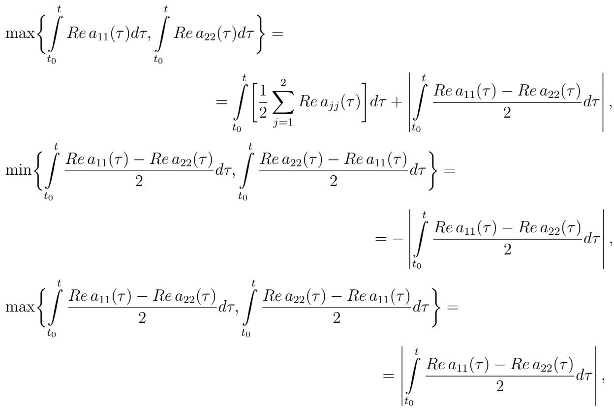
\[\begin{array}{r l} & {\min \biggl \{\int_ {t _ {0}} ^ {t} R e a _ {1 1} (\tau) d \tau , \int_ {t _ {0}} ^ {t} R e a _ {2 2} (\tau) d \tau \biggr \} =} \\& {\qquad = \int_ {t _ {0}} ^ {t} \biggl [ \frac {1}{2} \sum_ {j = 1} ^ {2} R e a _ {j j} (\tau) \biggr ] d \tau - \left| \int_ {t _ {0}} ^ {t} \frac {R e a _ {1 1} (\tau) - R e a _ {2 2} (\tau)}{2} d \tau \right|,} \end{array}\]
\[\begin{array}{r l r} & & {\max \biggl \{\int_ {t _ {0}} ^ {t} R e a _ {1 1} (\tau) d \tau , \int_ {t _ {0}} ^ {t} R e a _ {2 2} (\tau) d \tau \biggr \} =} \\& & {= \int_ {t _ {0}} ^ {t} \biggl [ \frac {1}{2} \sum_ {j = 1} ^ {2} R e a _ {j j} (\tau) \biggr ] d \tau + \left| \int_ {t _ {0}} ^ {t} \frac {R e a _ {1 1} (\tau) - R e a _ {2 2} (\tau)}{2} d \tau \right|,} \\& & {\min \biggl \{\int_ {t _ {0}} ^ {t} \frac {R e a _ {1 1} (\tau) - R e a _ {2 2} (\tau)}{2} d \tau , \int_ {t _ {0}} ^ {t} \frac {R e a _ {2 2} (\tau) - R e a _ {1 1} (\tau)}{2} d \tau \biggr \} =} \\& & {= - \left| \int_ {t _ {0}} ^ {t} \frac {R e a _ {1 1} (\tau) - R e a _ {2 2} (\tau)}{2} d \tau \right|,} \\& & {\max \biggl \{\int_ {t _ {0}} ^ {t} \frac {R e a _ {1 1} (\tau) - R e a _ {2 2} (\tau)}{2} d \tau , \int_ {t _ {0}} ^ {t} \frac {R e a _ {2 2} (\tau) - R e a _ {1 1} (\tau)}{2} d \tau {\biggr \}} =} \\& & {= \left| \int_ {t _ {0}} ^ {t} \frac {R e a _ {1 1} (\tau) - R e a _ {2 2} (\tau)}{2} d \tau \right|,} \end{array}\]
Remark 3.1. Let and be some continuous functions on and let , . Consider the system
. from (3.4) we will get (3.2). The theorem is proved.
\[\left\{
\begin{array}{l}
\phi^{\prime}(t) = a(t) \phi(t) + b(t) \psi(t); \\
\psi^{\prime}(t) = - b(t) \phi(t) + a(t) \psi(t), t \geq t_{0}.
\end{array}
\right.\]
For this system we have , . Therefore by Theorem 3.1 for its general solution the inequalities
\[| | (\phi (t _ {0}), \psi (t _ {0})) | | \exp \left\{\int_ {t _ {0}} ^ {t} R e a (\tau) d \tau \right\} \leq | | (\phi (t), \psi (t)) | | \leq | | (\phi (t _ {0}), \psi (t _ {0})) | | \exp \left\{\int_ {t _ {0}} ^ {t} R e a (\tau) d \tau \right\},\]
, are fulfilled. Hence
\[| | (\phi (t), \psi (t)) | | = | | (\phi (t _ {0}), \psi (t _ {0})) | | \exp \biggl \{\int_ {t _ {0}} ^ {t} R e a (\tau) d \tau \biggr \}, \qquad t \geq t _ {0},\]
and in this sense the estimates (3.2) are sharp.
Example 3.1. Consider the system
\[\left\{ \begin{array}{l l} \phi^{\prime}(t) = (- \lambda + \sin t) \phi(t) + t^{\alpha} \psi(t); \\ \psi^{\prime}(t) = - t^{\beta} \phi(t) + (- \mu + \cos t) \psi(t), \end{array} \right.\tag{3.5}\]
, where , , and are some real numbers. For this system ,
\[M (t) = t ^ {\frac {| \alpha - \beta |}{2}}, \mathcal {F} (t) = | \sqrt {2} + \lambda - \mu + (\lambda - \mu) t | + \int_ {\pi / 4} ^ {t} \left| \frac {\alpha - \beta}{4 \tau} + \frac {\lambda - \mu}{2} + \frac {\sqrt {2}}{2} \cos (\tau + \frac {\pi}{4}) \right| d \tau ,\]
. Using Theorem 3.1 it is easy to find the following regions of values of the parameters , , , for which the system (3.5) is asymptotically stable:
\[O _ {1} \equiv \{(\lambda , \mu , \alpha , \beta): \lambda + \mu > 3 | \lambda - \mu | + \sqrt {2}, \lambda > 0, \mu > 0 \};\]
\[O _ {2} \equiv \{(\lambda , \mu , \alpha , \beta): \lambda = \mu > \frac {\sqrt {2}}{2 \pi} \};\]
\[O _ {3} \equiv \{(\lambda , \mu , \alpha , \beta): \lambda + \mu > 3 | \lambda - \mu | > 3 ^ {\sqrt {}} 2, \lambda > 0, \mu > 0 \};\]
; and the following regions of values of parameters , , , for which system (3.5) is unstable:
\[O _ {5} \equiv \{(\lambda , \mu , \alpha , \beta): \lambda + \mu + 3 | \lambda - \mu | + \sqrt {2} < 0, \lambda < 0, \mu < 0 \};\]
\[O _ {6} \equiv \{(\lambda , \mu , \alpha , \beta): \lambda = \mu < - \frac {\sqrt {2}}{2 \pi} \};\]
\[O _ {7} \equiv \{(\lambda , \mu , \alpha , \beta): \lambda + \mu + 3 | \lambda - \mu | < 0, | \lambda - \mu | > \sqrt {2}, \lambda < 0, \mu < 0 \};\]
\[O _ {7} \equiv \{(\lambda , \mu , \alpha , \beta): \lambda + \mu + 3 | \lambda - \mu | < 0, | \lambda - \mu | = \sqrt {2}, \lambda < 0, \mu < 0, \alpha = \beta \};\]
It is not difficult to verify that the application of the estimates of Liapunov (see [4], p. 432), Yu. S. Bogdanov (see [4], p. 433) and estimate by freezing method (see [4], p. 441) to the system (3.5) give no result. The estimates by logarithmic norms and of S. M. Lozinski (see [4], pp. 435, 436) give result only for , , , . For comparison now we use the theorem of Wazevski to the system (3.5) (see [4], p. 434). By virtue of this theorem for each solution of the system (3.5) the following inequalities hold
\[| | (\phi (t), \psi (t)) | | \exp \left\{\int_ {\pi / 4} ^ {t} \omega_ {-} (\tau) d \tau \right\} \leq | | (\phi (t), \psi (t)) | | \leq\]
\[\leq | | (\phi (t), \psi (t)) | | \exp \biggl \{\int_ {\pi / 4} ^ {t} \omega_ {+} (\tau) d \tau \biggr \}, \quad t \geq \frac {\pi}{4},\tag{3.6}\]
where . If or , then from (3.6) does not follow neither asymptotic stability nor instability of the system (3.5) for every values of and .
Definition 3.1. A solution of the system (1.1), satisfying the condition B), is said to be a main (a nonprincipal, an ordinary) solution of the system (1.1), if , , where is a main (a nonprincipal, an ordinary) solution of the system (1.2).
Theorem 3.2. Let the condition be satisfied and let
\[\begin{array}{l} C) \int_ {t _ {0}} ^ {+ \infty} a _ {1 2} (t) \exp \biggl \{\int_ {t _ {0}} ^ {t} \Bigl [ a _ {2 2} (s) - a _ {1 1} (s) \Bigr ] d s \biggr \} d t = + \infty o r \\\qquad \qquad \qquad \qquad \qquad \qquad \qquad \qquad \qquad \qquad \qquad \qquad \qquad \qquad \qquad \qquad \qquad \qquad \qquad \qquad \qquad \qquad \qquad \qquad \qquad \qquad \qquad \qquad \qquad \qquad \qquad \qquad \qquad \qquad \\\qquad \qquad \qquad \qquad \qquad \qquad \qquad \qquad \qquad \qquad \qquad \qquad \qquad \qquad \qquad \qquad \qquad \qquad \qquad \qquad \qquad \qquad \qquad \qquad \qquad \qquad \qquad \qquad \qquad \qquad \qquad \qquad \qquad \end{array}\]
Then if:
i) is a nonprincipal solution of the system (1.1), then
\[D (\phi , \psi) m (t) \exp \left\{\int_ {t _ {0}} ^ {t} \left[ \frac {1}{2} \sum_ {j = 1} ^ {2} R e a _ {j j} (\tau) + \sqrt {a _ {1 2} (\tau) a _ {2 1} (\tau)} \right] d \tau - \mathcal {F} (t) \right\} \leq | \phi (t) | + | \psi (t) | \leq\]
\[\leq D (\phi , \psi) M (t) \exp \left\{\int_ {t _ {0}} ^ {t} \left[ \frac {1}{2} \sum_ {j = 1} ^ {2} R e a _ {j j} (\tau) + \sqrt {a _ {1 2} (\tau) a _ {2 1} (\tau)} \right] d \tau + \mathcal {F} (t) \right\}, \quad \psi t \geq t _ {0},\tag{3.7}\]
\[w h e r e D (\phi , \psi) \equiv \sqrt [ 4 ]{\left| \frac {a _ {2 1} (t _ {0})}{a _ {1 2} (t _ {0})} \right|} | \phi (t _ {0}) | + \sqrt [ 4 ]{\left| \frac {a _ {1 2} (t _ {0})}{a _ {2 1} (t _ {0})} \right|} | \psi (t _ {0}) |;\]
ii) is a main solution of the system (1.1), then
\[| \phi (t) | + | (t) | \leq\]
\[\leq \left(| \phi (t _ {0}) | + | \boldsymbol {\psi} (t _ {0}) |\right) \exp \left\{\int_ {t _ {0}} ^ {t} \left[ \frac {1}{2} \sum_ {j = 1} ^ {2} R e a _ {j j} (\tau) \right] d \tau + \left| \int_ {t _ {0}} ^ {t} \frac {R e a _ {1 1} (\tau) - R e a _ {2 2} (\tau)}{2} d \tau \right| \right\},\tag{3.8}\]
\[t \geq t _ {0};\]
iii) is an ordinary solution of the system (1.1), then
\[c _ {1} m (t) \exp \left\{\int_ {t _ {0}} ^ {t} \left[ \frac {1}{2} \sum_ {j = 1} ^ {2} R e a _ {j j} (\tau) + \sqrt {a _ {1 2} (\tau) a _ {2 1} (\tau)} \right] d \tau - \mathcal {F} (t) \right\} \leq | \phi (t) | + | \psi (t) | \leq\]
\[\leq c _ {2} M (t) \exp \bigg \{\int_ {t _ {0}} ^ {t} \bigg [ \frac {1}{2} \sum_ {j = 1} ^ {2} R e a _ {j j} (\tau) + \sqrt {a _ {1 2} (\tau) a _ {2 1} (\tau)} \bigg ] d \tau + \mathcal {F} (t) \bigg \}, \quad t \geq t _ {0},\tag{3.9}\]
where
Proof. Let be a solution of the system (1.1), and be the solution of the system (1.2) with , . Then by (3.1) we have
\[| \phi (t) | + | \psi (t) | = \exp \biggl \{\int_ {t _ {0}} ^ {t} R e a _ {1 1} (\tau) d \tau \biggr \} | u (t) | + \exp \biggl \{\int_ {t _ {0}} ^ {t} R e a _ {2 2} (\tau) d \tau \biggr \} | v (t) |, \qquad t \geq t _ {0}.\]
From here it follows
\[\exp \biggl \{\min \biggl \{\int_ {t _ {0}} ^ {t} R e a _ {1 1} (\tau) d \tau , \int_ {t _ {0}} ^ {t} R e a _ {2 2} (\tau) d \tau \biggr \} \biggr \} (| u (t) | + | v (t) |) \leq | \phi (t) | + | \psi (t) | \leq\]
\[\leq \exp \left\{\max \left\{\int_ {t _ {0}} ^ {t} R e a _ {1 1} (\tau) d \tau , \int_ {t _ {0}} ^ {t} R e a _ {2 2} (\tau) d \tau \right\} \right\} (| u (t) | + | v (t) |), \quad t \geq t _ {0},\]
or, which is the same,
\[\exp \biggl \{\int_ {t _ {0}} ^ {t} \biggl [ \frac {1}{2} \sum_ {j = 1} ^ {2} R e a _ {j j} (\tau) \biggr ] d \tau - \biggl | \int_ {t _ {0}} ^ {t} \frac {R e a _ {1 1} (\tau) - R e a _ {2 2} (\tau)}{2} d \tau \biggr | \biggr \} (| u (t) | + | v (t) |) \leq\]
\[\leq | \phi (t) | + | \psi (t) | \leq\]
\[\leq \exp \left\{\int_ {t _ {0}} ^ {t} \left[ \frac {1}{2} \sum_ {j = 1} ^ {2} R e a _ {j j} (\tau) \right] d \tau + \left| \int_ {t _ {0}} ^ {t} \frac {R e a _ {1 1} (\tau) - R e a _ {2 2} (\tau)}{2} d \tau \right| \right\} (| u (t) | + | v (t) |),\tag{3.10}\]
. Let be a real nonprincipal solution of the system (1.2). Then by virtue of Lemma 2.3 and (2.29) we have
\[\frac {\widetilde {D} E (t) \sqrt {P (t)}}{\sqrt {P (t _ {0})} r _ {H} ^ {-} (t)} \leq \sqrt {Q (t)} u _ {0} (t) + \sqrt {P (t)} v _ {0} (t) \leq \frac {\widetilde {D} E (t) \sqrt {Q (t)}}{\sqrt {Q (t _ {0})}} r _ {H} ^ {-} (t), \quad t \geq t _ {0},\tag{3.11}\]
\[\begin{array}{r l} & {\mathrm{where} \widetilde {D} \equiv \sqrt {Q (t _ {0})} u _ {0} (t) + \sqrt {P (t _ {0})} v _ {0} (t) = \sqrt {a _ {2 1} (t _ {0})} \phi (t _ {0}) + \sqrt {a _ {1 2} (t _ {0})} \psi (t _ {0}), E (t) \equiv} \\& {\equiv \exp \biggl \{\int_ {t _ {0}} ^ {t} \sqrt {P (\tau) Q (\tau)} d \tau \biggr \} = \exp \biggl \{\int_ {t _ {0}} ^ {t} \sqrt {a _ {1 2} (\tau) a _ {2 1} (\tau)} d \tau \biggr \}, t \geq t _ {0}. \mathrm{Obviously}} \\& {\min \{\sqrt {P (t)}, \sqrt {Q (t)} \} [ u _ {0} (t) + v _ {0} (t) ] \leq \sqrt {Q (t)} u _ {0} (t) + \sqrt {P (t)} v _ {0} (t) \leq} \\& {\qquad \leq \max \{\sqrt {P (t)}, \sqrt {Q (t)} \} [ u _ {0} (t) + v _ {0} (t) ], t \geq t _ {0}.} \end{array}\]
Therefore,
\[\begin{array}{r l} & {\min \bigg \{\frac {1}{\sqrt {P (t)}}, \frac {1}{\sqrt {Q (t)}} \bigg \} \bigg [ \sqrt {Q (t)} u _ {0} (t) + \sqrt {P (t)} v _ {0} (t) \bigg ] \leq u _ {0} (t) + v _ {0} (t) \leq} \\& {\qquad \leq \max \bigg \{\frac {1}{\sqrt {P (t)}}, \frac {1}{\sqrt {Q (t)}} \bigg \} \bigg [ \sqrt {Q (t)} u _ {0} (t) + \sqrt {P (t)} v _ {0} (t) \bigg ], \qquad t \geq t _ {0}.} \end{array}\]
From here and from (3.11) we will get
\[\widetilde {D} \min \left\{\sqrt [ 4 ]{\frac {P (t)}{Q (t)}}, \sqrt [ 4 ]{\frac {Q (t)}{P (t)}} \right\} \frac {E (t)}{\sqrt [ 4 ]{P (t _ {0}) Q (t _ {0})} r _ {H} (t)} \leq u _ {0} (t) + v _ {0} (t) \leq\]
\[\leq \widetilde {D} \max \biggl \{\sqrt [ 4 ]{\frac {P (t)}{Q (t)}}, \sqrt [ 4 ]{\frac {Q (t)}{P (t)}} \biggr \} \frac {E (t)}{\sqrt [ 4 ]{P (t _ {0}) Q (t _ {0})}} r _ {H} (t), \quad t \geq t _ {0}.\]
Therefore,
\[\frac {\widetilde {D} m (t)}{\sqrt [ 4 ]{a _ {1 2} (t _ {0}) a _ {2 1} (t _ {0})}} \exp \biggl \{- \biggl | \int_ {t _ {0}} ^ {t} \frac {R e a _ {1 1} (\tau) - R e a _ {2 2} (\tau)}{2} d \tau \biggr | \biggr \} \frac {E (t)}{r _ {H} (t)} \leq u _ {0} (t) + v _ {0} (t) \leq\]
\[\leq \frac {\widetilde {D} M (t)}{\sqrt [ 4 ]{a _ {1 2} (t _ {0}) a _ {2 1} (t _ {0})}} \exp \Biggl \{\left| \int_ {t _ {0}} ^ {t} \frac {R e a _ {1 1} (\tau) - R e a _ {2 2} (\tau)}{2} d \tau \right| \Biggr \} E (t) r _ {H} (t), \quad t \geq t _ {0}.\]
Taking into account the equalities , ,
from here we will get
\[D (\phi , \psi) \exp \biggl \{- \biggl | \int_ {t _ {0}} ^ {t} \frac {R e a _ {1 1} (\tau) - R e a _ {2 2} (\tau)}{2} d \tau \biggr | \biggr \} \frac {m (t) E (t)}{r _ {H} (t)} \leq | u (t) | + | v (t) |\]
\[\leq D (\phi , \psi) \exp \biggl \{\left| \int_ {t _ {0}} ^ {t} \frac {R e a _ {1 1} (\tau) - R e a _ {2 2} (\tau)}{2} d \tau \right| \biggr \} M (t) E (t) r _ {H} (t), \quad t \geq t _ {0}.\tag{3.12}\]
From here and from (3.10) it follows (3.7). The assertion i) is proved. Let us prove ii). Let be a main solution of the system (1.1). Then by (3.1) we have
\[\phi (t) = \phi (t _ {0}) \exp \biggl \{\int_ {t _ {0}} ^ {t} a _ {1 1} (\tau) d \tau \biggr \} u _ {0} (t), \psi (t) = \psi (t _ {0}) \exp \biggl \{\int_ {t _ {0}} ^ {t} a _ {2 2} (\tau) d \tau \biggr \} v _ {0} (t),\tag{3.13}\]
, where is the canonical main solution of the system (1.2). By (2.54) from C) it follows , . By (3.10) from here and from (3.13) it follows (3.8). The assertion ii) is proved. Let us prove iii). Let be an ordinary solution of the system (1.1). By (3.1) we have
\[\phi (t) = \exp \biggl \{\int_ {t _ {0}} ^ {t} a _ {1 1} (\tau) d \tau \biggr \} \biggl [ \lambda_ {0} u _ {0} (t) + \lambda_ {*} u _ {*} (t) \biggr ], \qquad t \geq t _ {0},\tag{3.14}\]
\[(t) = \exp \biggl \{\int_ {t _ {0}} ^ {t} a _ {1 1} (\tau) d \tau \biggr \} \biggl [ \lambda_ {0} v _ {0} (t) + \lambda_ {*} v _ {*} (t) \biggr ], \qquad t \geq t _ {0},\tag{3.15}\]
where and are the canonical main and canonical nonprincipal solutions of the system (1.2) respectively, and . Then by (2.29) and (2.52) we can deduce from C) that , , , j = 1, 2. By virtue of (3.10) from here, from (3.14) and (3.15) we obtain
\[\begin{array}{r l} & {\widetilde {c} _ {1} \exp \biggl \{\int_ {t _ {0}} ^ {t} \biggl [ \frac {1}{2} \sum_ {j = 1} ^ {2} R e a _ {j j} (\tau) \biggr ] d \tau - \biggl | \int_ {t _ {0}} ^ {t} \frac {R e a _ {1 1} (\tau) - R e a _ {2 2} (\tau)}{2} d \tau \biggr | \biggr \} [ u _ {0} (t) + v _ {0} (t) ] \leq} \\& {\qquad \leq | \phi (t) | + | \psi (t) | \leq} \end{array}\]
\[\leq \widetilde {c} _ {2} \exp \biggl \{\int_ {t _ {0}} ^ {t} \biggl [ \frac {1}{2} \sum_ {j = 1} ^ {2} R e a _ {j j} (\tau) \biggr ] d \tau + \biggl | \int_ {t _ {0}} ^ {t} \frac {R e a _ {1 1} (\tau) - R e a _ {2 2} (\tau)}{2} d \tau \biggr | \biggr \} [ u _ {0} (t) + v _ {0} (t) ],\]
. By (3.12) from here it follows (3.9). The assertion iii), and therefore, the theorem are proved.
Remark 3.2. Let and be the same as in Remark 3.1. Consider the system
\[\left\{
\begin{array}{l}
\phi^{\prime}(t) = a(t) \phi(t) + b(t) \psi(t); \\
\psi^{\prime}(t) = b(t) \phi(t) + a(t) \psi(t), t \geq t_{0}.
\end{array}
\right.\]
For this system we have , . Therefore by Theorem 3.2 for its each nonprincipal solution the inequalities
\[| \phi (t) | + | \psi (t) | = (| \phi (t _ {0}) | + | \psi (t _ {0}) |) \exp \biggl \{\int_ {t _ {0}} ^ {t} \Bigl [ R e a (\tau) + b (\tau) \Bigr ] d \tau \biggr \} \leq | \phi (t) | + | \psi (t) | \leq\]
\[\leq \left(| \phi (t _ {0}) | + | (t _ {0}) |\right) \exp \left\{\int_ {t _ {0}} ^ {t} [ R e a (\tau) + b (\tau) ] d \tau \right\}, \quad t \geq t _ {0},\]
are fulfilled. Hence
\[| \phi (t) | + | \boldsymbol {\psi} (t) | = (| \phi (t _ {0}) | + | \boldsymbol {\psi} (t _ {0}) |) \exp \biggl \{\int_ {t _ {0}} ^ {t} \Bigl [ R e a (\tau) + b (\tau) \Bigr ] d \tau \biggr \}, \qquad t \geq t _ {0},\]
and in this sense the estimates (3.7) are sharp.
Example 3.2. Let us consider the system
\[\left\{ \begin{array}{l l} \phi^{\prime}(t) = (- \lambda + \sin t) \phi(t) + t^{\alpha} \psi(t); \\ \psi^{\prime}(t) = t^{\beta} \phi(t) + (- \mu + \cos t) \psi(t), \end{array} \right.\]
(3.16)
, where , , and are some real constants. For this system the functions , and are the same, which are in the example 3.1. Applying Theorem 3.2 to (3.16) it is easy to find the following regions of parameters , , , for which Eq. (3.16) is asymptotically stable:
\[O _ {1} ^ {0} \equiv \{(\lambda , \mu , \alpha , \beta): \lambda + \mu > 3 | \lambda - \mu | + \sqrt {2}, \lambda > 0, \mu > 0, \lambda \neq \mu , \alpha + \beta < 0 \};\]
\[O _ {2} ^ {0} \equiv \left\{\left(\lambda , \mu , \alpha , \beta\right): \lambda + \mu > 3 | \lambda - \mu | + 2 + \sqrt {2}, \lambda > 0, \mu > 0, \lambda \neq \mu , \alpha + \beta = 0 \right\};\]
\[O _ {3} ^ {0} \equiv \{(\lambda , \mu , \alpha , \beta): \lambda + \mu > 3 | \lambda - \mu | > 3 \sqrt {2}, \lambda > 0, \mu > 0, \lambda \neq \mu , \alpha + \beta < 0 \};\]
\[O _ {4} ^ {0} \equiv \left\{\left(\lambda , \mu , \alpha , \beta\right): \lambda + \mu > 3 | \lambda - \mu | + 2 > 3 \sqrt {2} + 2, \lambda > 0, \mu > 0, \lambda \neq \mu , \alpha + \beta = 0 \right\};\]
\[O _ {5} ^ {0} \equiv \{(\lambda , \mu , \alpha , \beta): \lambda + \mu > 3 | \lambda - \mu | = 3 \sqrt {2}, \lambda > 0, \mu > 0, \lambda \neq \mu , \alpha = \beta < 0 \};\]
\[O _ {6} ^ {0} \equiv \{(\lambda , \mu , \alpha , \beta): \lambda + \mu > 3 | \lambda - \mu | + 1 = 3 \sqrt {2} + 2, \lambda > 0, \mu > 0, \lambda \neq \mu , \alpha = \beta = 0 \};\]
and the following regions of parameters , , , for which eq. (3.16) is instable:
\[\begin{array}{r l} & O _ {7} ^ {0} \equiv \{(\lambda , \mu , \alpha , \beta): \lambda \neq \mu , \alpha + \beta > 0 \}; \\& O _ {8} ^ {0} \equiv \{(\lambda , \mu , \alpha , \beta): \lambda + \mu + 3 | \lambda - \mu | + \sqrt {2} < 2, \lambda < 0, \mu < 0, \alpha + \beta = 0 \}; \\& O _ {9} ^ {0} \equiv \{(\lambda , \mu , \alpha , \beta): \lambda = \mu < - \frac {\sqrt {2}}{2 \pi} \}; \\& O _ {1 0} ^ {0} \equiv \{(\lambda , \mu , \alpha , \beta): \lambda + \mu + 3 | \lambda - \mu | < 2, | \lambda - \mu | \geq \sqrt {2}, \alpha + \beta = 0 \}. \end{array}\]
As in the case of the system (3.5) the application of the estimates of Liapunov, Yu. S. Bogdanov and estimate by freezing method to the system (3.16) give no result and the estimates by logarithmic norms and of S. M. Lozinski give result only for , , , . For the case or it is impossible by use of the theorem of Wazevski to verify neither asymptotic stability nor instability of system (3,16).

Great Britain Journals Press membership is an elite community of scholars, researchers, scientists, professionals and institutions associated with all the major disciplines. Great Britain memberships are for individuals, research institutions, and universities. Authors, subscribers, Editorial Board members, Advisory Board members, and organizations are all part of member network.
 For Authors
 For Institutions
 For Subscribers
Author Membership provide access to scientific innovation, next generation tools, access to conferences/seminars/symposiums/webinars, networking opportunities, and privileged benefits. Authors may submit research manuscript or paper without being an existing member of GBJP. Once a non-member author submits a research paper he/she becomes a part of "Provisional Author Membership".
Society flourish when two institutions Come together." Organizations, research institutes, and universities can join GBJP Subscription membershipor privileged "Fellow Membership" membership facilitating researchers to publish their work with us, become peer reviewers and join us on Advisory Board.
Subscribe to distinguished STM (scientific, technical, and medical) publisher. Subscription membership is available for individuals universities and institutions (print & online). Subscribers can access journals from our libraries, published in different formats like Printed Hardcopy, Interactive PDFs, EPUBs, eBooks, indexable documents and the author managed dynamic live web page articles, LaTeX, PDFs etc.