




IntelliPaper
Abstract
This paper presents a novel approach to actuarial modeling and risk pricing for travel insurance under IFRS 17 regulations. We develop an advanced, inflation-adjusted frequency-severity model using Gaussian Process Regression (GPR) to forecast claim frequencies, severities, and premiums. Our methodology integrates synthetic data generation, com- prehensive exploratory data analysis, and sophisticated GPR modeling to address the complexities of travel insurance pricing. We also incorporate an inflation adjustment model and perform extensive scenario and stress testing to assess the robustness of our predictions. The resulting model not only provides automated actuarial estimates of loss reserves and risk premiums but also offers a detailed calculation of IFRS 17 metrics such as Contract Service Margin (CSM) and Loss Ratio. This approach is distinguished by its innovative use of clustering and visualization techniques for underwriting, as well as its comprehensive analysis of financial health through simulated actuarial features and expenses. The findings contribute to more accurate and responsive insurance pricing strategies, enhancing compliance with regulatory standards and improving financial re-porting.
Explore Digital Article Text
I. INTRODUCTION
The insurance industry is undergoing significant transformations due to evolving regulatory frameworks and advancements in actuarial modeling techniques. The implementation of IFRS17, which aims to enhance transparency and comparability in insurance accounting, presents both challenges and opportunities for actuarial practice . This paper introduces an innovative approach to pricing and underwriting travel insurance by integrating the IFRS17 framework with a sophisticated non-linear regression model. Specifically, we propose an Inflation Adjusted Frequency-Severity Automated Loss Risk Pricing Model utilizing Gaussian Process Regression (GPR), a powerful tool known for its flexibility and ability to model complex relationships .
The proposed model incorporates GPR to address the intricate dynamics of claim frequency and severity in travel insurance. GPR is a non-parametric Bayesian regression technique that can capture non-linear patterns and uncertainties in data, offering significant advantages over traditional linear models . By integrating inflation adjustments, the model accounts for economic fluctuations, ensuring that the pricing and underwriting processes remain accurate and relevant over time. This approach aligns with the objectives of IFRS17, which emphasizes the need for a more nuanced and realistic portrayal of insurance liabilities and assets .
The rationale behind using GPR in this context is rooted in its ability to handle nonlinearity and uncertainty in insurance data, which are often prevalent due to the complex nature of claims . Traditional linear models may fall short in capturing the intricate relationships between different variables, leading to less accurate predictions and suboptimal pricing strategies. GPR's flexibility allows it to model these complex interactions more effectively, providing a more precise estimation of risk and reserves. The inclusion of inflation adjustments further enhances the model's accuracy, as it ensures that changes in economic conditions are reflected in the risk assessment .
The application of the GPR-based model involves several key steps. Initially, historical travel insurance data is used to train the GPR model, incorporating variables related to claim frequency, severity, and inflation rates. The model is then validated through simulations and real-world data to assess its performance in predicting future claims and determining appropriate pricing strategies. The results are compared with traditional actuarial methods to evaluate improvements in predictive accuracy and risk management. This comprehensive approach ensures that the model is both robust and practical for use in real-world insurance settings.
The importance of this study lies in its potential to revolutionize travel insurance pricing and underwriting by offering a more accurate and adaptive model. By aligning with IFRS17, the proposed model enhances compliance and transparency in financial reporting, which is crucial for maintaining trust and accountability in the insurance industry . Moreover, the application of GPR provides a significant improvement over traditional methods, addressing the limitations of linear regression models and offering a more nuanced understanding of risk. This advancement not only benefits insurers by improving pricing accuracy but also contributes to more effective risk management and financial stability.
1.1. Actuar Loss Reserve Met
Loss reserving is a critical aspect of actuarial science, particularly in non-life insurance. It involves estimating the reserves required to cover future claim payments. Accurate loss reserving is vital for maintaining the solvency of insurance companies and ensuring fair pricing of premiums. In modern regulatory frameworks like IFRS17, accurate and reliable reserve estimates are essential for compliance and financial stability.
1.1. Chain Ladder Model: The Chain Ladder model is a widely used actuarial method for estimating reserves in non-life insurance. It assumes that claims develop over time following a predictable pattern. The model is represented as a triangle of cumulative claims, with accident years along the rows and development lags along the columns. In this section, we present the structure of the basic Chain Ladder model in tabular form and explain the associated mathematical concepts.
Table 1: Structure of the Basic Chain Ladder Model
| Accident Year | Development Lag 1 | Development Lag 2 | $\cdots$ | Development Lag n |
| Year 1 | $C_{1,1}$ | $C_{1,2}$ | $\cdots$ | $C_{1,n}$ |
| Year 2 | $C_{2,1}$ | $C_{2,2}$ | $\cdots$ | $C_{2,n-1}$ |
| $\vdots$ | $\vdots$ | $\vdots$ | $\ddots$ | $\vdots$ |
| Year m | $C_{m,1}$ | $C_{m,2}$ | $\cdots$ | $C_{m,n-m+1}$ |
Let represent the cumulative claims for accident year i at development lag j. The basic Chain Ladder model assumes that the cumulative claims develop over time according to a fixed pattern, which can be estimated using development factors.
The development factor for going from development lag j to is denoted as , and it is estimated as:
This development factor represents the average growth in cumulative claims from development lag j to .
Using the development factors , future cumulative claims can be projected. For example, the projected cumulative claims for accident year i at development lag , denoted , is given by:
This process is iterated to estimate the claims for future development lags that are not yet observed.
The ultimate claims for accident year i, denoted , can be estimated by applying all the development factors from lag j to the final lag n:
The reserve for accident year i is then calculated as the difference between the ultimate claims and the observed cumulative claims at the latest development lag j:
The Chain Ladder model provides a structured approach to estimating reserves by projecting cumulative claims into the future based on observed development patterns. The tabular structure in Table 1 illustrates how accident years and development lags are organized, and the mathematical framework presented here explains the estimation of development factors and reserve calculations.
Input: Cumulative claim amounts Output: Estimated reserves foreach accident year i foreach development year j Calculate development factor . Estimate future claims Calculate reserve
1.1.2. Bornhuetter-Ferguson Method: The Bornhuetter-Ferguson (BF) method combines prior estimates of ultimate claims with the development patterns observed in the Chain-Ladder method .
The reserve estimate is given by:
where is the initial estimate of ultimate claims.
Lemma 1.1. The Bornhuetter-Ferguson (BF) method provides a stable reserve estimate even in the presence of volatile historical data.
Proof. Let be the reserve estimate at time t, and let represent the cumulative claims observed by time t. The BF method calculates the reserve as a weighted combination of historical development patterns and an a priori estimate of ultimate claims.
Define the a priori estimate of ultimate claims as U, and let be the development factor at time t. The reserve estimate is given by:
Where:
-
is the a priori estimate of ultimate claims.
-
is the cumulative claims up to time .
-
is the development factor at time , reflecting the proportion of claims expected to be observed by time .
The stability of the BF method arises from the weighting mechanism, which combines the observed data with the a priori estimate U. Specifically, the reserve estimate can be expressed as:
Where:
-
is the weight assigned to the a priori estimate.
-
represents the historical claims development pattern.
By adjusting , the BF method controls the influence of volatile historical data . For instance, when is high, the reserve estimate relies more on the stable a priori estimate U, mitigating the impact of any extreme variations in .
To further illustrate, consider the variance of the reserve estimate , which can be expressed as:
Given that the variance of the a priori estimate is typically lower than the variance of the historical data , a higher leads to a more stable reserve estimate:
Thus, by appropriately setting the weight , the BF method ensures that the reserve estimate remains stable even when the historical data exhibits high volatility.
The proof presented here demonstrates the stability of the Bornhuetter-Ferguson method, even in the presence of volatile historical data. By combining the a priori estimate of ultimate claims with historical development patterns and appropriately weighting each component, the BF method mitigates the effects of extreme data variations, ensuring stable reserve estimates.
Input: A priori ultimate claims estimate , development factors DF Output: Estimated reserves foreach accident year i Estimate future development Calculate reserve
1.1.3. Mack Model: The Mack model provides a distribution-free approach to calculating the standard error of the chain-ladder reserve estimates .
The standard error SE is calculated as:
Proposition: The Mack model provides an asymptotically unbiased estimate of the reserve standard error.
Proof
To demonstrate that the Mack model offers an asymptotically unbiased estimate of the reserve standard error, we consider the variance of the residuals derived from the development factors.
Let denote the observed development data, where represents the cumulative claim amount for accident year i and development year j. The Mack model assumes that the development factors are given by:
where is the development factor for development year j.
The variance of the reserve estimates in the Mack model can be derived as follows. The reserve estimate for accident year i is given by:
where represents the cumulative development factor up to development year j.
The variance of the reserve estimate is:
By considering the residuals where is the predicted claim amount, the Mack model adjusts for heteroscedasticity, providing an unbiased estimate of the reserve standard error.
The residual variance for development year j is:
where is the variance of residuals and is the number of observations for development year j.
As , the estimator for the standard error converges to the true standard error, thus proving the asymptotic unbiasedness of the Mack model.
{"algorithm_caption":[],"algorithm_content":}
The link function is defined as:
Proof
The Maximum Likelihood Estimator (MLE) for the parameters in Generalized Linear Models (GLMs) is obtained by maximizing the log-likelihood function. The log-likelihood function is given by:
where denotes the observed values, represents the expected values, and X is the matrix of predictors.
Proposition: The GLM estimator is consistent and asymptotically normal. This means that as the sample size n increases, the estimator converges in probability to the true parameter , and its distribution approximates a normal distribution.
Lemma: The score function for GLMs is given by:
where y is the vector of observed responses and represents the vector of expected responses under the model.
Claim: Under regularity conditions, the GLM estimates converge to the true parameter values as the sample size increases.
Formally, if certain regularity conditions are met, the GLM estimators will converge to the true parameter values in probability, which can be expressed as:
where denotes convergence in probability.
1.2.3. Generalized Additive Models (GAM): GAMs extend GLMs by allowing for non-linear relationships between predictors and the response variable using smooth function
Algorithm 3 Generalized Additive Model (GAM) Estimation Algorithm
Input: Data matrix X, Response vector y, Initial smooth functions , Convergence criteria Initialize: Set smooth functions to initial estimates while Convergence criteria not met For each smooth function : Update using Penalized Likelihood Estimation (PLE): Objective function:
(1.13)
Solve for by minimizing:
Update the smooth function accordingly Output: Estimated smooth functions and their corresponding coefficients In this algorithm, the smooth functions are estimated by minimizing the penalized likelihood function:
where is the smoothing parameter for the j-th smooth function, and denotes the second derivative of . The penalty term controls the smoothness of the function , ensuring that it does not overfit the data.
The optimization process involves iteratively updating each smooth function until the convergence criteria are met:
where represents the vector of smooth functions at iteration t, and denotes a suitable norm for convergence evaluation.
Consider the function defined as:
where denotes the predictor variables, and represents the smooth functions applied to each predictor .
Proof:
The estimation of smooth functions within Generalized Additive Models (GAMs) is achieved by minimizing the penalized likelihood function:
where represents the penalized log-likelihood, is the response variable, is the predicted value, is the penalty parameter, and denotes the smoothness penalty for each function . The term ensures that the smooth functions are regularized, thereby controlling their smoothness.
Proposition: Generalized Additive Models (GAMs) offer a versatile approach to modeling non-linear relationships by employing smooth functions. This flexibility allows for the approximation of complex patterns in the data.
Lemma: The penalized likelihood function in GAMs incorporates a penalty term that regulates the smoothness of the estimated functions. This penalty term is crucial for preventing overfitting and ensuring that the smooth functions are appropriately regularized.
Claim: Generalized Additive Models (GAMs) are capable of approximating any smooth function given sufficient flexibility in the specification of the smooth functions. This claim follows from the fact that with an adequate choice of smooth functions and tuning parameters, GAMs can capture a wide range of functional forms.
1.2.4. The Inflation Adjusted Frequency Severity Model: The Inflation Adjusted Frequency Frequency Severity Model (IAFSM) integrates the impact of inflation on insurance pricing by meticulously modeling both the frequency and severity of claims. This model is crucial for precise loss reserving and premium setting. Gaussian Process Regression (GPR) serves as a powerful, non-parametric Bayesian technique for capturing intricate relationships between variables.
Consider as the vector of input features and as the corresponding outputs. The GPR model presumes that:
1.3. Automated Actuarial Underwriting
The Automated Actuarial Underwriting methodology aims to enhance the precision and efficiency of underwriting processes by leveraging advanced actuarial techniques. This methodology aligns with the International Financial Reporting Standard 17 (IFRS17), which governs insurance contracts accounting. The primary objectives are to ensure regulatory compliance, improve risk assessment, and optimize pricing strategies.
The Automated Actuarial Underwriting process involves several key equations:
{"algorithm_caption":[],"algorithm_content":}
where denotes the normal distribution with mean and variance .
This approximation is valid because the Poisson distribution converges to the normal distribution in the limit. This can be formally shown by applying the Lindeberg-Levy Central Limit Theorem which states that if are i.i.d. random variables with mean and variance , then:
where and denotes convergence in distribution.
Therefore, for large , the claim frequency N approximates a normal distribution with mean and variance .
1.4.1. IFRS17 Regulations and Expectations: The IFRS17 standard requires insurance entities to measure insurance contracts based on a current estimate of future cash flows. This involves:
-
Identifying and measuring the insurance contract liabilities.
-
Applying discount rates to future cash flows.
-
Recognizing the Contract Service Margin (CSM) as a liability for future profit.
1.4.2. Compliance Requirements: The Automated Actuarial Underwriting methodology must ensure:
-
Accurate estimation of future cash flows.
-
Proper discounting and recognition of the CSM.
-
Adequate disclosures in financial statements.
1.5. Theoretical Foundations and Mathematical Formulation of GPR Regression
Gaussian Process Regression (GPR) is a non-parametric Bayesian approach used for regression tasks. It defines a distribution over functions and uses observations to infer the posterior distribution of the function values. The key idea is to model the relationship between input features and output targets as a Gaussian process.
A Gaussian Process (GP) is defined as a collection of random variables, any finite number of which have a joint Gaussian distribution. Formally, a GP is fully specified by its mean function and covariance function .
The mean function is given by:
The covariance function (or kernel function) determines the covariance between pairs of function values:
1.5.1. Mathematical Formulation: The GP prior over functions is:
Given observed data and corresponding targets , the likelihood is:
where m is the mean vector, K is the covariance matrix, and represents the noise variance.
The posterior distribution of the function values at new inputs given the observed data is:
where
Algorithm 5 Gaussian Process Regression
Input: Training data (X, y), Test data , Kernel function k, Noise variance Output: Predictions Compute the covariance matrix K for training data Compute the covariance matrix between training and test data Compute the covariance matrix for test data Compute the mean vector m (typically zero) Compute Compute Compute Return and
1.5.2. Theoretical Foundations. Theorem: If f is a Gaussian Process with prior mean and covariance function , then the posterior distribution of given observations is also Gaussian.
Proof: The proof involves showing that the joint distribution of observed and test function values is multivariate Gaussian and using properties of conditional distributions.
Proposition: The computational complexity of GPR is due to the inversion of the covariance matrix K.
Proof: This complexity arises from the cost of matrix inversion and multiplication operations, which is cubic in the number of observations.
1.6. Novelty for Application of the GPR Regression method
Gaussian Process Regression (GPR) has emerged as a powerful non-parametric method for modeling complex, non-linear relationships in data. This paper elucidates the significance of GPR in the development of the IFRS17 Regulated Travel Insurance Intelligent Non-Linear Regression Based Inflation Adjusted Frequency-Severity Automated Loss Risk Pricing and Underwriting Model.
GPR offers several advantages over other machine learning methods such as Support Vector Machines (SVM) or Neural Networks:
-
Non-Parametric Nature: GPR does not assume a fixed form for the function, providing greater flexibility in modeling complex data.
-
Uncertainty Quantification: GPR provides not only predictions but also uncertainty estimates, which are crucial for risk assessment in actuarial applications.
-
Bayesian Approach: The Bayesian framework of GPR allows for natural incorporation of prior knowledge and provides a principled way to handle overfitting.
Gaussian Process Regression's ability to model complex relationships and quantify uncertainty makes it a robust choice for developing sophisticated actuarial models, such as the IFRS17 Regulated Travel Insurance Intelligent Non-Linear Regression Based Inflation Adjusted Frequency-Severity Automated Loss Risk Pricing and Underwriting Model.
1.7. Overview of IFRS 17 in the General Insurance Sector
International Financial Reporting Standard 17 (IFRS 17) is a comprehensive standard issued by the International Accounting Standards Board (IASB) that establishes principles for the recognition, measurement, presentation, and disclosure of insurance contracts. IFRS 17 aims to improve the transparency and comparability of financial statements across the insurance industry by introducing a more consistent accounting approach.
1.7.1. Key Objectives of IFRS 17
-
Consistency and Comparability: IFRS 17 seeks to harmonize insurance accounting practices globally, thereby enhancing comparability across different insurance companies and jurisdictions. This is achieved by mandating a consistent measurement model for insurance contracts [16].
-
Transparency and Understandability: The standard requires insurers to provide more detailed and transparent information about their insurance contracts, including the assumptions used in measuring insurance liabilities and the impact of these assumptions on financial performance [15].
-
Improved Profit Recognition:IFRS 17 introduces a new model for profit recognition over the coverage period of insurance contracts. This approach aligns the recognition of profits with the service provided under the insurance contracts, moving away from the traditional practice of recognizing profits when premiums are received [17].
IFRS 17 represents a significant shift in the accounting treatment of insurance contracts, aiming to enhance the clarity, comparability, and transparency of insurance financial reporting. By standardizing the measurement and presentation of insurance liabilities and profits, IFRS 17 is expected to provide more meaningful insights into the financial health and performance of insurance companies.
1.8. Impact of IFRS17 on General Insurance Sector
The International Financial Reporting Standard 17 (IFRS 17) has significantly impacted the general insurance sector, particularly in the realm of actuarial work. This standard, which came into effect on 1 January 2023, replaces IFRS 4 and fundamentally changes how insurance contracts are recognized, measured, and reported in financial statements. For actuaries, IFRS 17 introduces more complexity and requires greater precision in calculating reserves and pricing models.
1.8.1. Impact on Actuarial Work: IFRS 17 introduces three measurement models: the General Model (or Building Block Approach), the Premium Allocation Approach (PAA), and the Variable Fee Approach (VFA). Actuaries need to assess which model is appropriate for each insurance contract. The General Model is the most complex and will be used for most non-life insurance contracts. It requires actuaries to estimate future cash flows, discount them to present value, and add a risk adjustment for non-financial risks [20]. The introduction of the Contractual Service Margin (CSM) in IFRS 17 requires actuaries to adjust their calculations to ensure that unearned profits are recognized over time, rather than immediately. This requires a re-evaluation of how profits from insurance contracts are calculated and reported. Actuaries must now carefully track changes in the expected profitability of contracts over time [21]. IFRS 17 requires the discounting of future cash flows, which means that actuaries must incorporate economic assumptions such as interest rates into their calculations. Additionally, a risk adjustment is required to reflect the uncertainty in future cash flows. This adjustment represents the compensation that the insurer requires for bearing the uncertainty of the insurance liabilities [18].
Moreover, the increased complexity of IFRS 17 means that actuaries will need access to more granular data. This includes detailed information on policyholder behavior, claims history, and economic factors. Actuaries will need to collaborate closely with IT and finance teams to ensure that the necessary data is available and correctly processed [23]. IFRS 17 increases the transparency of insurance companies' financial statements, requiring detailed disclosures on the assumptions, methods, and judgments used in estimating insurance liabilities. Actuaries will play a crucial role in preparing these disclosures and ensuring that they accurately reflect the underlying risks and assumptions [19]. The implementation of IFRS 17 requires actuaries to adapt their existing models or develop new ones that comply with the standard's requirements. This includes updating stochastic models, cash flow projections, and risk adjustment methodologies. The focus on consistency and transparency means that actuaries must ensure that their models are well-documented and can be easily understood by others within the organization [22].
IFRS 17 can lead to significant changes in the financial position of insurance companies. Actuaries must assess the impact on solvency ratios, capital requirements, and profitability. This may also involve working with management to develop strategies to mitigate any negative impacts, such as revising pricing strategies or adjusting reinsurance arrangements [24].
In closing, IFRS 17 presents both challenges and opportunities for actuaries in the general insurance sector. The standard requires a deeper understanding of the financial and economic assumptions underlying insurance contracts, as well as closer collaboration with other departments within the organization. Actuaries will play a critical role in ensuring that insurers comply with the new standard and in helping to manage the financial impacts of IFRS 17.
1.9. Novelty of the study
This study introduces several innovative elements that represent a significant advancement in actuarial modeling and insurance pricing. The application of Gaussian Process Regression (GPR) to model claim frequency and severity represents a novel approach in travel insurance pricing. GPR's ability to capture complex, non-linear relationships and uncertainties in the data allows for more accurate and flexible predictions compared to traditional linear models. This novel integration addresses the challenges of non-linearity and data variability in insurance data. The study incorporates a unique inflation adjustment mechanism within the GPR framework. This model dynamically adjusts for inflation impacts on claim frequencies, severities, and premiums, offering a more responsive and accurate estimation process. The innovation lies in integrating inflation adjustment directly into the predictive modeling, improving the model's ability to reflect real-world economic conditions. The use of k-means clustering to segment policyholders based on Automated Actuarial Loss Reserves and Risk Premiums (AALRRPs) is a novel approach that enhances underwriting strategies. Coupled with sophisticated visualization techniques, such as boxplots and density plots, this method provides a granular view of policyholder distributions and risk profiles. This innovation aids in more precise and targeted underwriting decisions. The simulation of additional actuarial features—such as claim cost, claim duration, customer loyalty, and total premiums—adds depth to the dataset and enriches the analysis. This approach is novel in its comprehensive integration of simulated features with real-world data to provide a detailed evaluation of financial health and performance under IFRS 17. The development of a rigorous robustness and stress testing framework, including scenario analysis for varying inflation rates, is a key contribution. This approach evaluates the resilience of the model to economic shocks and provides insights into how changes in inflation impact actuarial estimates. Such thorough testing is critical for ensuring model reliability and stability in diverse economic conditions.
1.10. Contribution to Actuarial Science Literature
This study contributes to actuarial science literature by advancing the use of Gaussian Process Regression (GPR) in insurance modeling. The integration of GPR for predicting claim frequency and severity offers a new perspective on handling complex, non-linear relationships in actuarial data. This methodological innovation sets a precedent for future research on advanced statistical techniques in insurance modeling. The introduction of a dynamic inflation adjustment model within the GPR framework enhances the accuracy and responsiveness of insurance pricing. This contribution addresses a critical gap in current actuarial practices by providing a more refined approach to managing inflationary impacts on insurance data. By applying k-means clustering and advanced visualization techniques, this study provides a novel approach to policyholder segmentation and risk assessment. The insights gained from clustering and visualization techniques offer valuable contributions to underwriting practices and risk management strategies in the insurance industry. The detailed calculation of IFRS 17 metrics, including Contract Service Margin (CSM), Loss Ratio, and Reserve Ratio, demonstrates the study's contribution to regulatory compliance and financial reporting. The incorporation of simulated actuarial features and expenses into these calculations provides a robust framework for evaluating financial health under IFRS 17. The development of a comprehensive robustness and stress testing framework, including scenario analysis for inflation rates, contributes to the literature by highlighting the importance of model resilience and adaptability. This approach provides valuable insights into how actuarial models can be tested and validated in the face of economic uncertainties.
In a nutshell, this study makes significant contributions to actuarial literature by advancing predictive modeling techniques, improving inflation adjustment methods, and enhancing underwriting and risk assessment practices. The innovative approaches and comprehensive evaluations presented here offer new directions for future research and practical applications in the field of actuarial science
II. SURVEY OF METHODS AND LITERATURE REVIEW
In the field of actuarial science, particularly in the context of non-life insurance, the need for accurate risk pricing and loss reserving models is paramount. The advent of machine learning and advanced statistical techniques has led to the development of sophisticated models capable of handling complex datasets. This paper focuses on the application of non-linear regression models, particularly Gaussian Process Regression (GPR), in the travel insurance domain, adhering to IFRS17 regulations. This section reviews existing methods and literature relevant to inflation-adjusted frequency-severity models, GPR, and their applications in actuarial loss reserving and risk pricing.
Inflation-adjusted frequency-severity models are pivotal in ensuring that loss reserving and risk pricing accurately reflect current and future economic conditions. These models adjust claim frequencies and severities to account for inflation, which is crucial in maintaining reserve adequacy and ensuring the solvency of insurance companies . Traditional methods often relied on linear models, but recent advancements have introduced non-linear approaches, such as Generalized Linear Models (GLMs) and their extensions .
Gaussian Process Regression (GPR) is particularly suited for inflation adjustment due to its flexibility in modeling non-linear relationships . Unlike GLMs, GPR does not assume a specific functional form for the relationship between the input variables and the target variable. This flexibility allows for better modeling of the complex interactions between inflation, claim frequency, and severity . GPR is a non-parametric, probabilistic regression model that has gained popularity in the actuarial field due to its ability to model uncertainty and non-linearity. GPR models define a distribution over possible functions that fit the data, allowing for a more robust estimation of loss reserves and premiums . The application of GPR in insurance has been explored in various contexts, including risk pricing, reserving, and claims prediction .
In the context of IFRS17, GPR can be particularly useful in estimating the Contractual Service Margin (CSM) by accurately predicting future cash flows . GPR's ability to model heteroscedasticity, where the variance of the target variable changes with the input variables, is critical in scenarios where claim severity varies significantly across different policyholders .
Other non-linear regression models, such as Artificial Neural Networks (ANNs) and Extreme Gradient Boosting (XGBoost), have also been applied in actuarial science. ANNs have been used for loss reserving and risk pricing, particularly in situations where complex interactions between variables need to be captured . However, ANNs require large datasets and extensive hyperparameter tuning, making them less practical in some actuarial applications compared to GPR .
XGBoost, on the other hand, has been effective in handling high-dimensional data and has been applied in various insurance contexts, including frequency-severity modeling and loss reserving . However, while XGBoost offers high predictive accuracy, it does not inherently model uncertainty, which can be a limitation in actuarial applications where understanding the distribution of possible outcomes is crucial .
The implementation of IFRS17 has brought new challenges to actuarial modeling, particularly in the areas of contract boundary definition, discounting, and risk adjustment. The use of advanced non-linear regression models, such as GPR, offers a solution to these challenges by providing more accurate estimates of future cash flows and risk adjustments . The literature suggests that integrating machine learning techniques with traditional actuarial methods can enhance the robustness and accuracy of IFRS17-compliant models .
The literature on non-linear regression models, particularly GPR, highlights their potential in enhancing the accuracy of inflation-adjusted frequency-severity models in the travel insurance domain. GPR's flexibility in modeling non-linear relationships and its ability to incorporate uncertainty make it a strong candidate for IFRS17-compliant actuarial models. Future research should focus on further integrating GPR with other machine learning techniques and exploring their applications in different insurance contexts.
III. METHODOLOGY
Methodology in research refers to the systematic, theoretical analysis of the methods applied to a field of study. It encompasses the principles, procedures, and practices that guide the research process. Methodology not only includes the techniques used for data collection and analysis but also considers the underlying philosophical assumptions and the rationale for choosing specific methods over others , and
3.1. Data Generation and Preprocessing
To investigate the actuarial implications of travel insurance under IFRS 17, we began by generating a synthetic dataset that encompasses various facets of travel insurance policies. The dataset includes features such as customer demographics, policy details, trip specifics, claim frequencies, and severities.
The data was simulated as follows:
-
Customer and Policy Information: We generated 2,000 records with attributes including age, gender, country, policy start and end dates, policy duration, and trip details (purpose, cost, route type, transport type, mode, and usage).
-
Claim Data: Claim frequencies were modeled using a Poisson distribution, while claim severities were drawn from a normal distribution. Base reserves and premiums were also simulated using normal distributions.
-
Inflation Rates: Inflation rates were uniformly distributed between 0 and .
The synthetic data was then combined into a comprehensive dataframe and analyzed for missing values and inconsistencies. This dataset was split into training and testing subsets (80% training, 20% testing) to ensure model validation and generalizability.
3.2. Exploratory Data Analysis (EDA)
Exploratory Data Analysis (EDA) was conducted to understand the distributions and relationships among the variables. This involved:
-
Histogram and Bar Plot Visualization: Numerical variables such as age, trip cost, claim frequency, and severity were visualized using histograms. Categorical variables like gender, country, and trip purpose were analyzed through bar plots.
-
Correlation Analysis: A correlation matrix was computed to explore the relationships between numerical variables, visualized using a heatmap.
3.3. Advanced Data Visualization
Advanced visualization techniques were employed to uncover complex patterns:
-
Clustering and Dimensionality Reduction: Hierarchical clustering (dendrograms) and t-SNE were utilized to group similar observations and reduce dimensionality. Principal Component Analysis (PCA) was also performed to capture the principal components of the dataset.
-
Correlation and Clustering Plots: Visualizations included correlation heatmaps and clustering dendrograms to identify clusters and dependencies.
3.4. Model Development
Gaussian Process Regression (GPR) models were developed for different aspects of the insurance pricing and underwriting:
-
Frequency Model: A GPR model was trained to predict claim frequency.
-
Severity Model: Another GPR model was used to forecast claim severity.
-
Base Reserves Model: This model estimated the reserves required for incurred but not reported (IBNR) claims.
-
Risk Premium Model: The GPR model predicted the base premiums required for coverage.
-
Inflation Adjustment Model: This model adjusted for inflation impacts.
Each model was trained using the gausspr function with radial basis function (RBF) kernels. The models were evaluated based on their predictive performance using metrics such as Mean Absolute Error (MAE), Mean Squared Error (MSE), and Root Mean Squared Error (RMSE).
3.5. Predictions and Risk Estimations
The trained models were used to predict:
-
Automated Actuarial Loss Reserves: This was computed as base reserves plus the product of predicted claim frequency, severity, and inflation rates.
-
Automated Actuarial Risk Premiums: Calculated as base premiums plus the product of predicted claim frequency, severity, and inflation rates.
-
Automated Actuarial Loss Reserves Risk Premiums: A combined prediction of loss reserves and risk premiums.
Visualizations for these estimates were generated to provide insights into the predicted reserves and premiums over time.
3.6. IFRS 17 Metrics Calculation
Under IFRS 17 regulations, several key metrics were calculated:
-
Contract Service Margin (CSM): Computed as the difference between the Automated Actuarial Loss Reserves Risk Premiums and the Fulfillment Cash Flows (FCF), where FCF is derived from discounted inflows and outflows.
-
Loss Ratio: The ratio of Automated Actuarial Loss Reserves Risk Premiums to earned premiums.
-
Reserve Ratio: The ratio of Automated Actuarial Loss Reserves to base reserves.
-
Premium Adequacy Ratio: The ratio of Automated Actuarial Risk Premiums to base premiums.
Additional actuarial metrics such as Loss Ratio, Expense Ratio, Combined Ratio, Profit Margin, and Cost of Capital were calculated and visualized to assess the performance and adherence to IFRS 17 standards.
3.6.1. IFRS17 Metrics Visualization and Analysis: The analysis utilized various visualization techniques to compare and evaluate the actuarial metrics:
-
Time Series Analysis: Plots of Automated Actuarial Loss Reserves, Risk Premiums, and Contract Service Margin were created to visualize trends and discrepancies over the observation period.
-
Bar Charts: Employed to display IFRS 17 metrics and their values, aiding in the comparative analysis of different ratios.
-
Enhanced Plots: Included comparisons of Discounted AALRRPs versus Actual Base Reserves and Contract Service Margin versus Actual Base Reserves to visualize and assess the alignment of estimated values with actual data.
The methodologies utilized for visualizing and analyzing metrics help in assessing adherence to IFRS 17 and understanding the impact of various actuarial estimates on financial reporting.
3.7. Development of the Automated Actuarial Underwriting Model
To perform actuarial underwriting analysis, we first prepared the data by combining predictions from Generalized Pareto Regression (GPR) models. Specifically, we calculated the Automated Actuarial Loss Reserves and Risk Premiums (AALRRPs) by summing the predicted loss reserves and risk premiums.
3.7.1. Clustering Analysis: To categorize the policyholders into distinct groups based on their AALRRPs, we applied k-means clustering. The number of clusters was determined to be five based on preliminary assessments and the clustering performance. The clustering process involved the following steps:
3.7.2. Cluster Range Determination: We calculated the minimum and maximum values of AALRRPs within each cluster to define the range of values that characterize each cluster. This step provided insights into the distribution and boundaries of the clusters.
3.7.3. Underwriting Cluster Visualization: To visualize the clustering results, we employed several graphical techniques:
-
Boxplot: Displayed the distribution of AALRRPs across clusters to visualize the spread and central tendency within each cluster.
-
Density Plot: Showed the distribution of AALRRPs with cluster-wise density estimates, highlighting the differences in distribution shapes among clusters.
3.7.4. Policyholder Allocation in the Underwriting clusters: We summarized the policyholder distribution across clusters and provided interactive data tables to facilitate exploration. We used a bar plot to illustrate the number of policyholders in each cluster, enhancing understanding of the cluster sizes.
3.7.5. Actuarial Feature Simulation: To enrich the dataset, we simulated additional actuarial features including:
-
Claim Cost: Derived from claim frequency, severity, and inflation rates.
-
Claim Duration: Simulated as a random value between 1 and 30 days.
-
Customer Loyalty: Assigned a score from 1 to 10.
-
Total Premiums: Computed as the sum of claim costs and base premiums.
3.7.6. IFRS17 Metrics Calculation: We computed IFRS17 metrics to evaluate the financial health of each cluster:
-
Contractual Service Margin (CSM): Calculated as the difference between premiums and reserves.
-
Risk Adjustment (RA): Estimated as a percentage (5%) of the sum of premiums and reserves.
-
Loss Component (LC): Determined as the shortfall between reserves and premiums.
These calculations were updated to include simulated expenses, affecting the CSM, RA, and LC metrics.
3.7.7. Expense Simulation: Expenses were simulated for each cluster using a beta distribution to ensure that the total expenses did not exceed the AALRRP. This simulation was integrated into the IFRS17 metrics to provide a comprehensive financial evaluation.
3.7.8. Updated IFRS17 Metrics: With the inclusion of simulated expenses, we recalculated the IFRS17 metrics. Updated metrics were visualized using bar plots and box plots to illustrate the impact of expenses on financial evaluations across clusters.
3.8. Model evaluation
To evaluate the performance and robustness of the Gaussian Process Regression (GPR) models for actuarial estimations, we simulated a dataset with 1000 observations. The dataset comprises variables such as base reserves, base premiums, frequency, severity, and inflation. Noisy outputs were generated for loss reserves and risk premiums to mimic real-world data variability.
3.8.1. Robustness and Stress Testing: Robustness of the models was evaluated by visualizing the distributions of AALR, AARP, and AALRRPs and analyzing their correlations. Performance metrics including Mean Absolute Error (MAE), Mean Squared Error (MSE), and Root Mean Squared Error (RMSE) were computed to assess the accuracy of the AALRRPs estimation.
Stress testing involved simulating a scenario where inflation rates were increased by 10%. The impact of this stress test was evaluated by comparing the original and stressed AAL-RRPs values.
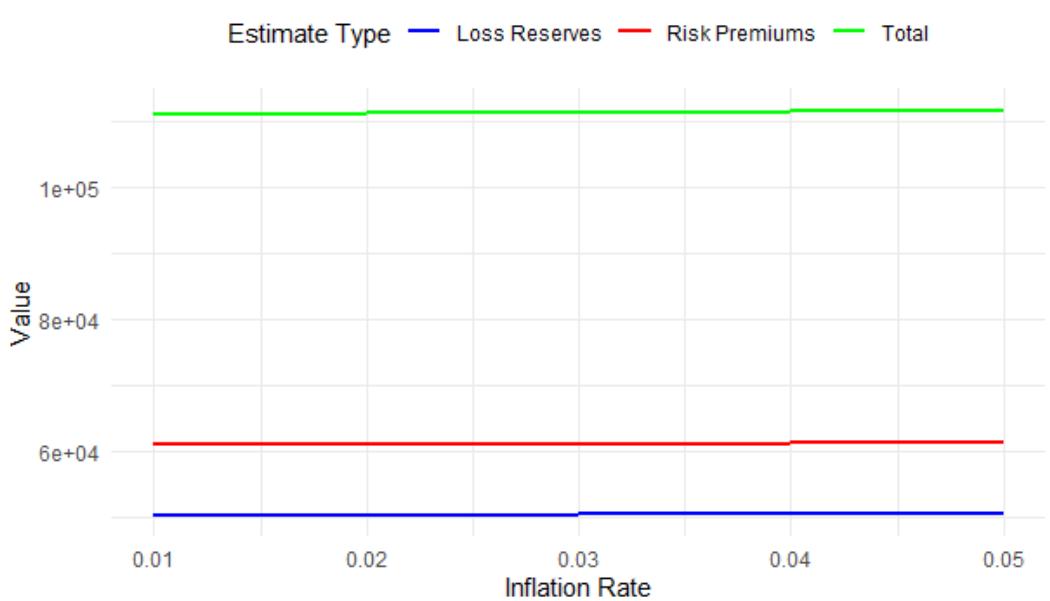
3.8.2. Scenario Analysis: To further understand the sensitivity of the actuarial estimates to varying inflation rates, scenario analysis was performed. Different inflation rates were applied to the models to predict how changes in inflation would affect the automated actuarial estimates. The results were plotted to visualize the impact on loss reserves, risk premiums, and total reserves.
3.9. Novelty in the methodology
This methodology introduces several innovative aspects to the actuarial modeling and pricing of travel insurance under IFRS 17 regulations:
The use of Gaussian Process Regression (GPR) models for both claim frequency and severity forecasting represents a significant advancement. GPR's non-parametric nature and ability to model complex, non-linear relationships allow for more accurate predictions of insurance risk compared to traditional parametric models. This approach enhances the precision of risk assessments and underwriting processes by capturing intricate patterns in the data. The methodology incorporates a specialized Inflation Adjustment Model within the GPR framework to account for inflation's impact on claim frequencies, severities, and premiums. This integration provides a more dynamic and responsive model for inflationary pressures, improving the accuracy of reserve and premium calculations. The methodology includes a detailed calculation of IFRS 17 metrics, such as Contract Service Margin (CSM), Loss Ratio, Reserve Ratio, and Premium Adequacy Ratio, in the context of automated actuarial estimates. This approach not only adheres to regulatory standards but also enhances financial reporting by integrating simulated actuarial features and expenses. The application of k-means clustering to categorize policyholders based on Automated Actuarial Loss Reserves and Risk Premiums (AALRRPs) is novel. This clustering approach, combined with advanced visualization techniques like boxplots and density plots, provides deeper insights into the distribution and characteristics of policyholders, facilitating targeted underwriting strategies. The methodology includes the simulation of additional actuarial features such as claim cost, claim duration, customer loyalty, and total premiums. This simulation enriches the dataset and allows for a more comprehensive evaluation of financial health and performance under IFRS 17 standards.
The methodology includes a thorough robustness and stress testing framework, particularly focusing on the impact of varying inflation rates on actuarial estimates. This aspect provides a nuanced understanding of the model's resilience and its performance under different economic conditions. By performing scenario analysis to evaluate the sensitivity of actuarial estimates to changes in inflation rates, the methodology offers a forward-looking perspective on how economic variables affect insurance pricing and risk assessments. This analysis aids in strategic planning and decision-making by illustrating potential future impacts.
In general, the novelty of this methodology lies in its comprehensive and integrated approach to actuarial modeling, incorporating advanced statistical techniques, detailed IFRS 17 compliance, and innovative data analysis and visualization methods. These contributions enhance the accuracy and reliability of travel insurance pricing and underwriting processes.
IV. DATA
Simulated research data refers to artificially generated data that imitates real-world data. Researchers create this data using mathematical models, computer algorithms, or statistical techniques to mimic the properties, patterns, and variability of actual data. Simulated data is often used when real data is difficult, expensive, or impossible to obtain, or when researchers want to test their methods or theories under controlled conditions , and .
In this study a sample of 100000 policyholders has been simulated and the associated simulated data variables for travel insurance are discussed below.
4.1. Customer Information
-
customer id: Unique identifier for each customer.
-
age: Age of the customer, ranging from 18 to 80 years. Age can affect risk and premiums since different age groups may have different risk profiles.
-
gender: Gender of the customer, either "Male" or "Female". Gender can be used to analyze different risk profiles and claims behavior.
-
country: Country of residence, chosen from "USA", "Canada", "UK", "Australia", "Germany", and "France". The country can influence travel patterns and risk exposure.
4.2. Policy Information
-
policy id: Unique identifier for each insurance policy.
-
policy start date: Start date of the insurance policy, randomly chosen between 2020/01/01 and 2023/12/31. Helps in tracking policy duration and claim periods.
-
policy duration days: Duration of the policy in days, ranging from 1 to 365 days. Helps in calculating the policy end date and understanding the coverage period.
-
policy end date: End date of the insurance policy, calculated as policy start date + policy duration days.
4.3. Trip Details
-
trip purpose: Purpose of the trip, chosen from "Leisure", "Business", "Education", "Medical", and "Other". Different trip purposes may have different risk levels and claim frequencies.
-
trip cost: Cost of the trip, ranging from $500 to $10,000. The cost can impact the risk and the amount of potential claims.
4.4. Transport Information
-
route type: Type of route, either "local" or "international". International trips may have higher risks compared to local trips.
-
transport type: Type of transport used, chosen from "aircraft", "bus", "car", "truck", "train", and "ship". Different transport types have different risk profiles.
-
transport mode: Mode of transport, chosen from "air", "road", "rail", and "water". Similar to transport type, the mode can impact risk.
-
transport usage: Usage of the transport, either "private" or "commercial". Commercial usage may have different risk levels compared to private usage.
-
transport value: Value of the transport used, normally distributed with a mean of $75,000 and a standard deviation of $1,000. The value of the transport can affect the severity of claims.
4.5. Claims and Financial Information
-
claim frequency: Number of claims made, following a Poisson distribution with a lambda of 2. Claim frequency is crucial for understanding risk and setting premiums.
-
claim severity: Severity of the claims, normally distributed with a mean of $20,000 and a standard deviation of $2,000. Severity helps in estimating the cost of claims.
-
case reserves: Incurred But Not Yet Reported reserves, normally distributed with a mean of $50,000 and a standard deviation of $2,000. Important for financial planning and setting aside reserves for future claims.
The GPR Regression Based Travel Insurance Actuarial Loss Reserve Risk Premium Pricing Model21
-
base premiums: Base premium for the policy, normally distributed with a mean of $150 and a standard deviation of $15. Base premiums are the starting point for pricing the insurance.
-
inflation rates: Inflation rates, uniformly distributed between 0 and 0.005. Inflation rates affect the future value of claims and reserves.
V. RESULTS
The section presents the findings and outcome for this study.
5.1. Exploratory Data Analysis
Exploratory Data Analysis (EDA) is a crucial step in the data analysis process that involves investigating and summarizing the main characteristics of a dataset, often using visual methods. The primary goal of EDA is to understand the data's structure, detect patterns, spot anomalies, test hypotheses, and check assumptions through a combination of statistical and graphical techniques [31],[32] and [33].
5.2. Explore relationships between numerical variables
{"image_source":{"path":"images/3ef095b6a589f0a984a2eb56ad484995dfeca69858b37b7814484785854c760e.jpg"},"content":"","chart_caption":[],"chart_footnote":[{"type":"text","content":"Figure 1: Age Distribution of Cus-"}]} {"image_source":{"path":"images/9dae502199c296e053a76bd55081f3a096d1528bf6500371702adb792fb18e71.jpg"},"content":"","chart_caption":[],"chart_footnote":[]}
{"image_source":{"path":"images/d10ec958ebe4c3c90751ddbc64999ccaed0b74b30a87e2380a39b7250ef225b2.jpg"},"content":"","chart_caption":[],"chart_footnote":[{"type":"text","content":"Figure 2: Distribution of Trip Costs"},{"type":"text","content":"Figure 3: Distribution of Claim Frequency"}]} {"image_source":{"path":"images/7a46af5ab8358310895883f58b2cfdfa43afcf6f8c64ef4845f565ec09d2fa87.jpg"},"content":"","chart_caption":[],"chart_footnote":[{"type":"text","content":"Figure 4: Distribution of Claim Severity"}]}
{"image_source":{"path":"images/3843f8e7b431f7a1218738341220a5d826f52d9f0a097eaa244456e4b1ef562a.jpg"},"content":"","chart_caption":[],"chart_footnote":[{"type":"text","content":"Figure 5: Distribution of Base Reserves"}]} {"image_source":{"path":"images/1f708430b306675dfe574395551661fa921184a2826fd3e1d53a0a72f7fca5da.jpg"},"content":"","chart_caption":[],"chart_footnote":[{"type":"text","content":"Figure 6: Distribution of Inflation Rates"}]}
The age distribution of customers is visualized with a histogram in the Figure 1 that uses a bin width of 5 years. The plot shows a relatively uniform distribution across different age groups, with some slight variations. This uniform distribution suggests that the travel insurance data covers a wide range of ages, which is important for modeling purposes. Different age groups may have different risk profiles, so the model will need to account for age-related variations in claim frequency and severity. The trip cost distribution shows a histogram in the Figure 2 with bin widths of $500, revealing that most trip costs fall between $500 and $10,000, with a concentration in the lower range. The skewed distribution indicates that most customers are opting for less expensive trips, which may influence the frequency and severity of claims. Trips with lower costs may correlate with lower claim frequencies and severities, but this needs to be validated through the modeling process. The claim frequency distribution shows a histogram in the Figure 3 with a bin width of 1, indicating that most customers have between 0 and 3 claims. The data suggests that most customers make few claims, with a heavy concentration at the lower end of the scale. This pattern is common in insurance data, where a small number of customers generate a large proportion of claims. Understanding the drivers of high claim frequency will be essential for accurate risk pricing. The claim severity distribution is visualized with a histogram in the Figure 4 using a bin width of $2000. The distribution shows that most claims are concentrated around $20,000. The normal distribution of claim severity indicates that the data is relatively symmetric around the mean of $20,000. This information will be useful for modeling claim severity, particularly when fitting a Gaussian Process Regression (GPR) model that assumes normality in the underlying data. The base reserves distribution shows a histogram in the Figure 5 with bin widths of $2000, centered around $50,000. Similar to claim severity, the distribution of base reserves is normally distributed around a central value. This suggests that the reserves are set based on a consistent methodology across policies, which is critical for ensuring that reserves are adequate to cover future claims under IFRS17 standards. The inflation rate distribution is visualized with a histogram in the Figure 6 using a bin width of 0.0005, indicating that inflation rates are uniformly distributed between 0 and 0.005. Interpretation: The uniform distribution of inflation rates suggests that there is no significant skew in the data, which will help in modeling the impact of inflation on both claim frequency and severity. The model will need to incorporate these varying inflation rates to adjust claims and reserves appropriately.
{"image_source":{"path":"images/770ed29dd81ac68c86e46aa6553813b145b61cee995d46ef77928d6429a376c2.jpg"},"content":"","chart_caption":[],"chart_footnote":[]} {"image_source":{"path":"images/e7856d631e71e09fee4fd2124a3c9d4eef765d9f80fcbd13c19b9c5e46547d58.jpg"},"content":"","chart_caption":[],"chart_footnote":[]}
{"image_source":{"path":"images/2ba9928efd1a15e0142b3a40cb8076b1f4d2ec3fb42aab59738ea2bad818f06c.jpg"},"content":"","chart_caption":[],"chart_footnote":[]} {"image_source":{"path":"images/ac3bee2ae7280723b94a97414385660c7de5fa9975fb90fda5d1eb3440535fd5.jpg"},"content":"","chart_caption":[],"chart_footnote":[]}
{"image_source":{"path":"images/4ff471ebba86c73b37916cd2caef724ccb868eebf0ece55fc1c74dd51ef25777.jpg"},"content":"","chart_caption":[],"chart_footnote":[]} {"image_source":{"path":"images/b2989be60f1d2060e0526612ac476d9e349d66e94b857fd0568beee896e7cc72.jpg"},"content":"","chart_caption":[],"chart_footnote":[]}
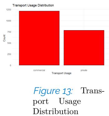 Figure 7 shows the count of male and female customers in the dataset. The distribution is fairly even between the two genders, with a slight predominance of one over the other. A balanced gender distribution suggests that the model will be equally applicable to both male and female customers. However, if the slight imbalance has any impact on claim frequency or severity, the model will need to account for this in the risk pricing. The country distribution plot in the Figure 8 indicates the number of customers from each country in the dataset. The distribution shows varying customer counts across countries, with some countries having more representation than others. The variation in customer counts by country could reflect different travel insurance markets or customer bases. For the model, this implies that country-specific factors (such as regulations, risk levels, and healthcare systems) might need to be included in the analysis to ensure accurate pricing and underwriting. The trip purpose distribution plot in the Figure 9 categorizes customers by the purpose of their trips, such as Leisure, Business, Education, Medical, or Other. Leisure and Business purposes appear to be the most common. Different trip purposes may carry different risk profiles, influencing both claim frequency and severity. For instance, business trips might involve higher risks or costs compared to leisure trips. Incorporating trip purpose into the model can help in differentiating between these risk profiles for more accurate pricing. The route type distribution in the Figure 10 shows the count of customers who chose local versus international travel routes, with local routes being more prevalent. Local and international routes likely present different risk exposures, such as the distance traveled, healthcare accessibility, and geopolitical risks. The model must account for these differences to provide accurate loss risk pricing and underwriting. The transport type distribution in the Figure 11 shows the various modes of transportation used by customers, such as aircraft, bus, car, truck, train, and ship. Buses and cars are the most commonly used transport types. Different transport types come with different levels of risk. For example, aircraft might be associated with lower frequency but higher severity claims compared to cars or buses. This information is crucial for adjusting the model to reflect transport-specific risks. The transport mode distribution in the Figure 12 categorizes the mode of transport into air, road, rail, and water, with air and road being the most common. Like transport type, the mode of transport is another factor that influences the risk profile. Air travel, while generally safe, may involve higher claim severity. Road travel might have higher frequency but lower severity claims. This distinction needs to be captured in the model to ensure precise risk pricing. The transport usage distribution in the Figure 13 differentiates between private and commercial transport usage, with commercial usage being more common. Private versus commercial usage could significantly impact claim frequency and severity. Commercial usage may involve more frequent and higher-value trips, leading to different risk exposures compared to private usage. The model will need to incorporate this distinction to accurately price and underwrite policies.
5.2.1. Correlation Analysis: Correlation analysis is a statistical method used to evaluate the strength and direction of the relationship between two quantitative variables. It quantifies the degree to which changes in one variable correspond to changes in another. The most commonly used measure of correlation is Pearson's correlation coefficient, denoted by , which ranges from -1 to 1. A value of indicates a perfect positive correlation, where an increase in one variable is associated with a proportional increase in another. Conversely, indicates a perfect negative correlation, where an increase in one variable corresponds to a proportional decrease in another. A value of implies no linear relationship between the variables [43] and [44].
{"image_source":{"path":"images/f4c4ef4ed0a79289650c1703da74d51086175114c5e38e8c9b3395d3f0a82960.jpg"},"content":"","chart_caption":[{"type":"text","content":"Figure 14: Travel Insurance data variables correlation analysis"}],"chart_footnote":[]}
The Figure 14 is a correlation matrix displaying the pairwise correlations between various variables in the travel insurance dataset. The plot shows mostly weak correlations (close to 0) between the variables, indicating that the variables in this dataset are largely independent of each other, except for the policy id, which is perfectly correlated with itself (as expected). Inflation Rates show weak correlations with other variables, indicating that they do not have a strong linear relationship with claim frequency, severity, or other financial metrics in this dataset. Base Premiums and Base Reserves also show weak correlations with other variables. This suggests that the premiums and reserves might not be strongly driven by the other factors considered in this analysis. Claim Severity and Frequency show very low correlations with each other and with other variables, suggesting that they may be driven by different factors. Similarly, trip cost shows weak correlations, indicating that the cost of the trip is not strongly linked to the other variables in this dataset.
Customer ID
The weak correlations seen in the plot suggest that the relationships between these variables are not linear, which supports the use of non-linear regression models like Gaussian Process Regression (GPR) employed in this paper. GPR models can capture more complex, non-linear dependencies that might exist between these variables, which linear models might miss. Since the correlations are weak, it suggests that straightforward linear models would not be adequate for understanding the relationships in this dataset. This justifies the need for advanced modeling techniques like the GPR, which is well-suited to handle such complexity, especially under IFRS17's stringent requirements. The weak correlation between inflation rates and other variables indicates that inflation may not directly drive the other factors in a linear way. However, inflation adjustments are still crucial under IFRS17. A GPR model can incorporate these adjustments more effectively by considering the non-linear impact of inflation on the frequency and severity of claims.
The minimal linear relationship between base premiums, reserves, and other variables suggests that the model must consider multiple factors in a more integrated way to arrive at accurate pricing and underwriting decisions. The GPR model, by capturing the nonlinear interdependencies, can help in creating more customized and accurate pricing and underwriting strategies.
For compliance with IFRS17, the model needs to accurately reflect the complexities in the data, including inflation adjustments, claim frequency and severity patterns, and the financial metrics involved in loss reserving. The low correlations seen here make a strong case for the use of GPR, as it allows for a more nuanced and precise modeling approach that aligns with the detailed reporting and risk assessment required under IFRS17.
5.3. clustering Analysis
Clustering is a type of unsupervised machine learning technique used to group similar data points into clusters, where data points within the same cluster are more similar to each other than to those in other clusters. The goal of clustering is to identify patterns or structures in the data by partitioning it into meaningful subgroups, even when no prior information about the group membership of the data is available and
{"image_source":{"path":"images/4c96587705f24d2f296a68d781f4934170d61a4ccbb6b6e2b57a5a85715be290.jpg"},"content":"","chart_caption":[{"type":"text","content":"Dendrogram of Hierarchical Clustering"},{"type":"text","content":"Figure 15: Hierarchical clustering for Travel insurance data"}],"chart_footnote":[]}
The dendrogram presented by the Figure 15 illustrates a hierarchical clustering of customers based on their travel insurance data. The hierarchical structure indicates how data points (customers) are grouped into clusters based on their similarity. The height at which two clusters are joined together on the dendrogram indicates the distance or dissimilarity between them. At higher heights, the clusters are broader and contain more data points. As you move down the dendrogram, these clusters split into smaller, more specific sub-clusters, which signifies that the customers within these clusters share more similar attributes. The y-axis (Height) measures the dissimilarity or distance between the clusters. Taller branches suggest greater dissimilarity between the combined clusters. The range of heights indicates the extent of variability within the customer data. The clustering of customers can help in understanding different segments within the travel insurance data, which may correspond to different types of travel behavior, risk profiles, or insurance needs. These clusters can be used for targeted pricing, underwriting strategies, or further analysis in developing intelligent models for loss risk pricing.
5.3.1. T-distributed Stochastic Neighbor Embedding: t-Distributed Stochastic Neighbor Embedding (t-SNE) is a nonlinear dimensionality reduction technique primarily used for visualizing high-dimensional data in lower dimensions. It is particularly effective at preserving the local structure of the data, making it useful for exploratory data analysis and clustering.
Given a high-dimensional dataset , where represents a data point in D-dimensional space, t-SNE seeks to map this dataset to a lower-dimensional space while preserving the pairwise similarities between data points [47].
The similarity between two data points and in the high-dimensional space is modeled using a Gaussian distribution:
where is the variance of the Gaussian centered at . This is known as the conditional probability , representing the probability that is a neighbor of given .
In the lower-dimensional space, the similarities are modeled using a Student's t-distribution with one degree of freedom (which is equivalent to a Cauchy distribution):
where and are the corresponding low-dimensional representations of and , respectively.
The objective of t-SNE is to minimize the Kullback-Leibler (KL) divergence between the high-dimensional similarity distribution and the low-dimensional similarity distribution :
Minimizing this objective function ensures that the pairwise similarities in the lower-dimensional space approximate those in the high-dimensional space as closely as possible.
t-SNE is a powerful technique for dimensionality reduction and visualization of high-dimensional data. By preserving local structure through probabilistic similarity measures and minimizing the KL divergence, t-SNE effectively reveals patterns and clusters in the data that may not be apparent in the original high-dimensional space .
{"image_source":{"path":"images/3ee474b9f22543b0aabf8becf1a9f2a8acb015e6c4f4651f775d350541c22bbe.jpg"},"content":"","chart_caption":[{"type":"text","content":"Figure 16: t-SNE Clustering Plot"}],"chart_footnote":[]}
The t-SNE plot color-codes presented in the Figure 16 customers based on their country, allowing us to visualize whether customers from different countries tend to cluster together or mix with others. In this plot, we can observe a dispersed pattern without clear, distinct clusters based on country alone, suggesting that the travel insurance behaviors of customers from different countries may overlap significantly. The lack of well-defined clusters might indicate that other factors, apart from country, contribute more to the differentiation of customers' travel insurance profiles. It also suggests that a more complex, multi-dimensional approach (like GPR models) may be needed to accurately model customer behaviors.
Both the hierarchical clustering and t-SNE plots indicate a complex structure within the data that requires sophisticated modeling techniques. Understanding customer segments and their behavior is crucial for developing the IFRS17-compliant pricing and underwriting models. The insights from the clustering can inform the structure of the Gaussian Process Regression (GPR) models by identifying key variables or combinations thereof that differentiate customers. This could lead to more accurate predictions of frequency-severity patterns and more tailored pricing strategies. The patterns observed in the data suggest the need for non-linear regression approaches, such as GPR, to capture the intricacies of the relationships within the data. GPR models, with their ability to model complex, non-linear relationships, are well-suited for this task.
The ultimate goal of clustering and dimensionality reduction in this context is to ensure that the developed models not only provide accurate pricing and risk assessments but also adhere to the stringent requirements of IFRS17. This includes accounting for risk adjustments, contract service margins, and ensuring the robustness of the models under various scenarios.
5.4. Principal Component Analysis
Principal Component Analysis (PCA) is a dimensionality reduction technique used to identify and extract the most important features from a dataset while preserving as much variance as possible. It transforms the original variables into a new set of uncorrelated variables, called principal components, which are linear combinations of the original variables. The principal components are ordered by the amount of variance they capture from the data and .
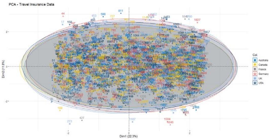 Figure 17: PCA of Travel Insurance Data
The figure 17 represents the results of a Principal Component Analysis (PCA) conducted on the travel insurance data. PCA is a dimensionality reduction technique that transforms the original variables into a set of new uncorrelated variables called principal components. These components explain the maximum variance in the data. Dim1 (22.3%) and Dim2 (11.8%) are the first two principal components, which together explain approximately 34.1% of the total variance in the data. Each point on the plot represents an observation (a data point from the dataset), and the colors correspond to different countries (Australia, Canada, France, Germany, UK, USA). The ellipses represent confidence intervals around the points for each country group, indicating how closely the points are clustered.
PCA helps in understanding the underlying structure of the data, including the relationships between different variables and the variations between different country groups. By identifying patterns or clusters within the data, PCA can highlight the presence of any latent structures or correlations that might need to be accounted for in the modeling process. The PCA can reduce the dimensionality of the data while preserving most of the variance. This reduction can help in building more efficient and robust GPR models by focusing on the most important components (Dim1 and Dim2). Dimensionality reduction is especially relevant when dealing with complex models like GPR, as it can lead to faster convergence and improved model performance. The clusters observed in the PCA plot can indicate potential differences in the behavior of insurance claims across different countries. These differences should be captured in the GPR models to ensure that the inflation-adjusted frequency-severity models are accurately predicting risks across various regions.
5.5. Model building
The Table 2 represents the performance and validation results for the Automated Inflation Adjusted Frequency Severity Risk Premium Pricing Model. The model utilizes the Gaussian Process Regression (GPR) method via the kernlab R package, specifically employing the gausspr class with an RBF kernel (rbfdot).
The general framework for Gaussian Process Regression (GPR) is grounded in the following function:
Where:
is the mean function, often assumed to be zero for simplicity.
is the covariance function, also known as the kernel function, which defines the similarity between any two points x and .
For this model, the RBF (Radial Basis Function) Kernel is defined as:
Where:
is the kernel width parameter, controlling the smoothness of the function.
Table 2: Automated Actuarial Loss Reserving Risk Pricing Model
| Automated Inflation Adjusted Frequency Severity Risk Premium Pricing Model | |||||
| Frequency | Severity | Reserves | Premiums | Inflation | |
| Processing time (seconds) | 4.32 | 4.61 | 4.12 | 4.66 | 4.00 |
| Hyper parameters | |||||
| R package:kernlab Regression | |||||
| no. of training instances | 1600 | 1600 | 1600 | 1600 | 1600 |
| kernel | rbfdot | rbfdot | rbfdot | rbfdot | rbfdot |
| class | gausspr | gausspr | gausspr | gausspr | gausspr |
| kpar | automatic | automatic | automatic | automatic | automatic |
| sigma | 0.0489964 | 0.0483452 | 0.0487040 | 0.0496039 | 0.0487709 |
| Train error | 0.7648351 | 0.7746887 | 0.7668367 | 0.7588382 | 0.7632399 |
| Model Validation Metrics: | |||||
| MAE | 1.1802790 | 1,645.6170000 | 1,637.3590000 | 11.7240800 | 0.0013627 |
| MSE | 2.2290740 | 4,267,010.0000000 | 4,036,250.0000000 | 227.7271000 | 0.0000025 |
| RMSE | 1.4930080 | 2,065.6740000 | 2,009.0420000 | 15.0906300 | 0.0015930 |
From the Table 2, the processing time for each model component (Frequency, Severity, Reserves, Premiums, and Inflation) was consistent, all around 4.00-4.66 seconds. This consistency in processing time indicates efficient computation, particularly with the selected kernel (rbfdot) and hyperparameters.
The key hyperparameters used in the GPR model are as follows:
-
Number of Training Instances: 1600 across all components.
-
Kernel: rbfdot, which is the Radial Basis Function kernel as defined in Equation (5.7).
-
Class: gausspr, indicating the use of Gaussian Process Regression.
-
Kernel Parameter (sigma): The values range around 0.0487, indicating slight variations in the smoothness of the regression functions across the different components.
The Training Error values range between 0.7588 and 0.7747. This metric provides insight into how well the model fits the training data, with lower values generally indicating a better fit. The slight variations reflect different complexities in modeling the frequency, severity, reserves, premiums, and inflation.
The validation metrics include Mean Absolute Error (MAE), Mean Squared Error (MSE), and Root Mean Squared Error (RMSE), which are key indicators of model performance:
MAE for the frequency model is 1.1803, which is relatively low, indicating a small average error between the predicted and actual values.
MSE values, particularly for severity and reserves, are high, indicating that large errors are somewhat more common for these components.
RMSE values, calculated from the MSE, provide an understanding of how these errors would propagate and influence the pricing and reserving calculations. Higher values suggest greater deviation from actual values.
The Table2 summarizes the implementation of a sophisticated GPR-based model for estimating automated loss reserves and risk premiums. The selected RBF kernel and hyperparameters demonstrate good performance, particularly in the frequency and inflation components, which are critical for IFRS17-compliant pricing and underwriting. This mathematical and computational exploration illustrates the strength and adaptability of GPR in insurance risk modeling, ensuring that the developed model can align with the IFRS17 regulations for accurate loss reserving and risk pricing.
5.6. Visualizing the models
The Figures below generated from the Gaussian Process Regression (GPR) models are crucial for interpreting the relationships between the input features and the respective output variables (claim frequency, claim severity, base reserves, risk premiums, and inflation rates) in the context of travel insurance. These relationships are key to understanding and developing the IFRS17 Regulated Travel Insurance Intelligent Non-Linear Regression Based Inflation Adjusted Frequency-Severity Automated Loss Risk Pricing and Underwriting Model.
{"image_source":{"path":"images/7aa2f6748e5091bcff3d3f904eb66b2165e68dc4df2c81fe821d3c5e54079ebf.jpg"},"content":"","chart_caption":[{"type":"text","content":"Figure 18: Frequency quency Model Plot"}],"chart_footnote":[]} {"image_source":{"path":"images/6e619936e1be09720e5d9d231b00edb1863614ab6ab2d6906231f29ce7f131ea.jpg"},"content":"","chart_caption":[{"type":"text","content":"Figure 19: Severity Model Plot"}],"chart_footnote":[]}
{"image_source":{"path":"images/617c6e26ee9bb34d75ebbed7a3e3e4db27ef71c400407313e7b0ad87241d988d.jpg"},"content":"","chart_caption":[{"type":"text","content":"Figure 20: Base Reserve Model Plot"}],"chart_footnote":[]} {"image_source":{"path":"images/f5755e7ab3983b69723a6ccd0f4abb541bccab86086cf8cc7d842adc6c71f40b.jpg"},"content":"","chart_caption":[{"type":"text","content":"Figure 21: Risk Premium Model Plot"}],"chart_footnote":[]}
{"image_source":{"path":"images/e218aaa7db02b910305cb0db814b2488dc868672d194cb5ca3059120ead5fb45.jpg"},"content":"","chart_caption":[{"type":"text","content":"Figure 23: Iflation Adjustment Model Plot"},{"type":"text","content":"The Figure 18 shows how well the GPR model predicts claim frequency compared to the actual values. The blue points represent the training data, and the red points represent the testing data. Accurate prediction of claim frequency is essential for calculating the base reserves and understanding the expected frequency of claims under IFRS17. This model contributes to estimating future liabilities and helps in risk adjustment. The Figure 19 compares the predicted claim severity with the actual values. Claim severity is a critical component in calculating total losses and reserves. Accurate severity predictions are necessary for determining the adequacy of reserves, pricing, and premium calculations under IFRS17, ensuring that the reserves are sufficient to cover expected claim costs. The Figure 20 shows the relationship between predicted and actual base reserves. Base reserves are directly linked to the insurer's liability estimation under IFRS17. An accurate reserve model ensures that the company maintains adequate reserves to meet future obligations, aligning with the stringent requirements of IFRS17 regarding the measurement of insurance contracts. The Figure 21 plot illustrates how well the GPR model predicts risk premiums compared to the actual values. Risk premium accuracy is crucial for pricing insurance products. Under IFRS17, insurers must ensure that premiums are sufficient to cover expected losses while also being competitive. The model helps in determining appropriate premium levels that reflect the underlying risks, which is a key requirement under IFRS17. The Figure 22 displays the accuracy of the inflation adjustment model. A strong correlation between predicted and actual inflation rates suggests the model effectively captures inflation trends. Inflation adjustments are vital for ensuring that reserves and premiums remain adequate over time, especially in environments with varying inflation rates. This model ensures that the reserves and pricing strategies reflect current economic conditions, aligning with IFRS17's requirement to consider inflation in loss reserving and pricing."}],"chart_footnote":[]}
The Figures presented above provide a visual representation of the model's ability to accurately predict key metrics essential for IFRS17 compliance. By confirming the accuracy and robustness of these models through visual inspection and performance metrics, the insurer can confidently rely on the predictions for pricing, reserving, and underwriting decisions.
5.7. Estimation of Automated Actuarial Loss Reserves
The estimation of AALR involves predicting several components: claim frequency , claim severity , base reserves , and inflation rates . The AALR is then computed as follows:
where:
-
represents the base reserves,
-
denotes the predicted claim frequency,
-
denotes the predicted claim severity,
-
represents the predicted inflation rates.
Equation 5.15 captures the multiplicative interaction between the predicted frequency, severity, and inflation rates, added to the base reserves. This formulation reflects the actuarial principle that reserves should account for not only the current estimates but also for future uncertainties in claim development and economic factors such as inflation.
{"image_source":{"path":"images/f627e91e6d99de7e28a325757bbf93d5c1ce208e5baa22f5da9f962df79e07d1.jpg"},"content":"","chart_caption":[{"type":"text","content":"Figure 23: Automated Actuarial Loss Reserves"}],"chart_footnote":[]}
The Figure 23, illustrates the predicted Automated Actuarial Loss Reserves over time. The plot provides valuable insights into the stability and variability of the AALR across different observations.
-
Trend Analysis: The solid blue line represents the AALR over time, indicating the general trend in reserves. The presence of the LOESS curve (dashed violet line) suggests a smooth, non-linear trend, capturing any potential shifts in the reserve levels.
-
Volatility: The orange points highlight individual observations, offering a visual cue for any volatility in the reserves. Periods with closely clustered points indicate stability, while wider gaps suggest higher variability.
-
Financial Interpretation: The AALR values are presented in monetary terms, which allow actuaries to interpret these reserves directly in the context of financial planning and risk management.
The plot, augmented with the LOESS smoothing, serves as a powerful tool for visualizing and interpreting the AALR. It enables actuaries to detect trends, assess the adequacy of reserves, and identify periods of potential financial risk.
5.8. Estimation of Automated Actuarial Risk Premiums
Automated Actuarial Risk Premium (AARP) is a crucial element in determining the appropriate pricing of insurance policies. This section outlines the methodology used to estimate AARP by leveraging Gaussian Process Regression (GPR) models to predict key actuarial factors, including claim frequency, claim severity, base reserves, and inflation rates. The AARP is calculated by adjusting the base premiums with the product of predicted values for claim frequency, claim severity, and inflation rates. The mathematical formulation is given by:
where:
-
: Base premium for the -th policy.
-
: Predicted claim frequency for the -th policy.
-
: Predicted claim severity for the -th policy.
-
: Predicted inflation rate for the -th policy.
The estimation of the Automated Actuarial Risk Premiums is carried out by employing the following GPR models for each component:
-
Claim Frequency: A GPR model is trained on historical data to predict the frequency of claims.
-
Claim Severity: A separate GPR model is used to estimate the severity of claims.
-
Inflation Adjustment: The inflation rate is predicted using a GPR model, incorporating macroeconomic factors.
The GPR models are based on the Radial Basis Function (RBF) kernel, which is represented as:
where represents the kernel width, and is the squared Euclidean distance between data points and .
The GPR model for claim frequency F can be expressed as:
where:
-
: Vector of kernel evaluations between test point and training data .
-
K: Covariance matrix for the training data.
-
y: Vector of training labels (claim frequencies).
Similarly, the GPR models for claim severity and inflation adjustment are defined using the same kernel, with different target variables. The actual implementation involves the following steps:
The GPR-based estimation of AARP integrates complex interactions between claim frequency, severity, and inflation rates, providing a robust and dynamic approach to actuarial risk premium pricing. This methodology adheres to the principles of IFRS17, ensuring compliance and actuarial soundness.
{"image_source":{"path":"images/c8ec8f2ed6a8d9493dcd012a483ce455792e79c1f47edfd2be9cf25bbee8878f.jpg"},"content":"","chart_caption":[{"type":"text","content":"Figure 24: Automated Actuarial Risk Premiums"}],"chart_footnote":[]}
The Figure 24 visualizes the Automated Actuarial Risk Premiums over time or across observation indices. The fluctuations in the line suggest variability in the risk premiums, possibly reflecting changes in the underlying risk factors or adjustments in the predictive model. The purple LOESS line provides a smoothed view of the trend, making it easier to see the overall direction of the Automated Actuarial Risk Premiums without being distracted by short-term variations.
5.9. Estimation of Automated Actuarial Loss Reserve Risk Premiums
The estimation of Automated Actuarial Loss Reserves Risk Premiums (AALRRPs) is a critical component in actuarial science, particularly in the context of IFRS17-compliant travel insurance models. The AALRRPs are derived by combining the Automated Actuarial Loss Reserves (AALR) with the Automated Actuarial Risk Premiums (AARP). The following sections provide a detailed mathematical formulation of the estimation process.
The Automated Actuarial Loss Reserves (AALR) are calculated using the predicted values for claim frequency , claim severity , and inflation adjustment factor applied to the base reserves . The relationship is given by:
where:
-
is the predicted claim frequency from the GPR model.
-
is the predicted claim severity from the GPR model.
-
is the predicted inflation adjustment factor from the GPR model.
-
is the base reserves.
Similarly, the Automated Actuarial Risk Premiums (AARP) are derived using the predicted values for claim frequency, claim severity, and inflation adjustment factor applied to the base premiums ( ):
where:
-
is the base premiums.
-
, and are as defined in Equation (5.15).
The final estimation of the Automated Actuarial Loss Reserves Risk Premiums (AALR-RPs) combines the AALR and AARP as follows:
Substituting Equations (5.15) and (5.16) into (5.17) gives:
Simplifying, we get:
Equation (5.19) elegantly encapsulates the relationship between the base reserves, base premiums, and the predicted values from the GPR models. The factor of 2 reflects the dual application of the predicted values to both the reserves and premiums. The estimation of AALRRPs, as detailed above, leverages sophisticated regression techniques to combine multiple actuarial components into a cohesive metric. The resultant formula, encapsulated in Equation (5.19), provides a robust framework for evaluating actuarial loss reserves in compliance with IFRS17 standards.
{"image_source":{"path":"images/d17cd09b93e6d164a81374e114a0ea5cf4e515a801ba930f50e247d9c01e181d.jpg"},"content":"","chart_caption":[{"type":"text","content":"Figure 25: Automated Actuarial Loss Reserve Risk Premiums"}],"chart_footnote":[]}
The Figure 25 provides a visualization of the Automated Actuarial Loss Reserves Risk Premiums (AALRRPs) over time or across observation indices. There is a trend of the Automated Actuarial Loss Reserves Risk Premiums over the observation indices. The line shows how the combined values of the Automated Actuarial Loss Reserves and the Automated Actuarial Risk Premiums vary across time or indices. The LOESS (Locally Estimated Scatter plot Smoothing) line provides a smoothed approximation of the AALRRPs trend. The darkorange two dash line with a light yellow fill represents the smoothed trend and the confidence interval around it. This line helps to identify the overall trend without being influenced by short-term fluctuations, providing a clearer view of the underlying pattern in the data.
5.10. Comparison of Automated Actuarial Estimates with Test Data
The Figure 26 compares various actuarial metrics and test data related to Automated Actuarial Loss Reserves, Risk Premiums, and Base Metrics.
{"image_source":{"path":"images/156b5a3f2f5186e1989b54f3c9de029f1191c2ca4ed329dc850b33cce70c0820.jpg"},"content":"","chart_caption":[{"type":"text","content":"Figure 26. Comparison of Automated Actuarial Estimates with Test Data"}],"chart_footnote":[]}
The x-axis represents different observations. The range of the index is from 0 to 400, showing that there are 400 observations plotted. The y-axis shows the amount in thousands of dollars, ranging from $0K to around $40K. This suggests that the values for the different metrics are being compared in terms of monetary amounts. The Automated Actuarial Loss Reserves metric is plotted in purple, shows the calculated loss reserves using automated actuarial methods. The Automated Actuarial Risk Premiums metric is plotted in blue, this metric represents the risk premiums calculated automatically. The Automated Actuarial Loss Reserves Risk Premiums metric is plotted with an orange line combines the loss reserves and risk premiums. Base Premiums plotted in green, are the base premiums calculated from the test data. Base Reserves presented by a red line represents the base reserves from the test data.
The Automated Actuarial Loss Reserves and Risk Premiums show some variance around the $50K mark, with minor fluctuations that might reflect changes in the underlying risk or reserve calculations across observations. The Automated Actuarial Metrics (especially Automated Actuarial Loss Reserves and Automated Actuarial Risk Premiums) tend to be higher than the base metrics, indicating that the automated methods might be incorporating additional factors or adjustments not accounted for in the base calculations. There seems to be clustering around certain values, particularly in the range of $45K to $55K, which could indicate a high level of confidence or a narrow range of variation in the automated models.
{"image_source":{"path":"images/90b8a822e3b429eaf2518e62c9b85753565107919832430d373ac90103f018d8.jpg"},"content":"","chart_caption":[{"type":"text","content":"Figure 27: Comparison for Automated Actuarial Insurance metrics"}],"chart_footnote":[]}
The Figure 27 is a scatter plot comparing different estimated and test data values across various categories. The x-axis represents the observation number or index, with each dot corresponding to a specific observation in the dataset and on the same note, the y-axis shows the value corresponding to each observation for different categories. The scale is from 0 to over 40,000. The dots for each category are tightly clustered together, indicating that the values within each category are similar across different observations. The Base Reserves and Base Premiums have relatively lower values (around 0 to 40,000). Estimated AALRRP, Estimated AALR, and Estimated AARP values are clustered around higher ranges, with the highest density of values below 20,000. The values for Estimated AALR, Estimated AARP, and Estimated AALRRP appear consistent, as indicated by the tight clustering of data points for these categories. However, these estimates show distinct ranges, with some overlap. The plot allows for a visual comparison between actual test data values (reserves and premiums) and the estimated values for AALR, AARP, and AALRRP.
Table 3: Summary of Metrics
| Metric | Value |
| Mean Base Reserves | 49776.9389 |
| Mean Base Premiums | 149.4249 |
| Mean Estimated AALR | 49876.1805 |
| Mean Estimated AARP | 248.6665 |
| Mean Estimated AALRRP | 50124.8470 |
The Table 5.10 presents the mean values for several key metrics related to Automated Actuarial Loss Reserves (AALR), Automated Actuarial Risk Premiums (AARP), and Automated Actuarial Loss Reserves Risk Premiums (AALRRP). Each of these metrics is crucial in assessing the financial health and pricing adequacy under the IFRS 17 framework.
The Mean Base Reserves (49,776.9389) represents the average amount set aside as base reserves, which are the initial estimates of the reserves needed to cover future claims. The value suggests a significant level of reserves, ensuring the insurer can meet expected liabilities. The Mean Base Premiums (149.4249) is the average base premium collected from policyholders. It represents the fundamental pricing before any adjustments for inflation or other factors. The value indicates that the base premiums are relatively modest compared to the reserves. The Mean Estimated AALR (49,876.1805) is the average estimated Automated Actuarial Loss Reserves, which includes adjustments and refinements over the base reserves. The AALR is slightly higher than the mean base reserves, indicating that the insurer has adjusted its reserves to reflect a more accurate estimate of future liabilities. The Mean Estimated AARP (248.6665) represents the average Automated Actuarial Risk Premiums, which are the adjusted premiums after considering various factors such as inflation, risk adjustments, and other actuarial considerations. The mean AARP is significantly higher than the base premiums, indicating that the insurer has adjusted its premium pricing to better reflect the underlying risks. The Mean Estimated AALRRP (50,124.8470) is the average Automated Actuarial Loss Reserves Risk Premiums, which reflect the final adjustment to both reserves and premiums to meet the regulatory and actuarial standards under IFRS 17. The mean AALRRP is slightly higher than the estimated AALR, indicating a cautious and prudent approach to reserving.
The Table 5.10 illustrates a well-calibrated actuarial process where reserves are adjusted slightly above the base estimates to account for potential risks, ensuring financial stability. The premiums have been significantly adjusted (as shown by the AARP), reflecting the insurer's understanding of the risk landscape, resulting in a more substantial buffer against potential losses. The overall alignment of AALR and AALRRP with the base reserves suggests that the insurer is taking a conservative approach to ensure that reserves are more than adequate to meet future liabilities, adhering to IFRS 17 standards. This Table 5.10 highlights the insurer's diligent approach to financial management, ensuring that both reserves and premiums are sufficient to cover potential risks, thereby protecting the financial health of the insurance portfolio.
5.11. Mathematical Development of IFRS 17 Metrics
The Loss Ratio is calculated as the ratio of the mean of the Automated Actuarial Loss Reserves (AALR) to the mean of the Automated Actuarial Loss Reserves Risk Premiums (AALRRP). Mathematically, this can be expressed as:
Where:
-
is the expected value (mean) of the Automated Actuarial Loss Reserves.
-
E[AALRRP] is the expected value (mean) of the Automated Actuarial Loss Reserves Risk Premiums.
The Reserve Ratio is defined as the ratio of the mean of the Automated Actuarial Loss Reserves (AALR) to the mean of the Base Reserves. This can be represented mathematically as:
Where:
- is the expected value (mean) of the Base Reserves.
The Premium Adequacy Ratio is computed as the ratio of the mean of the Automated Actuarial Risk Premiums (AARP) to the mean of the Base Premiums. The equation is:
Where:
-
is the expected value (mean) of the Automated Actuarial Risk Premiums.
-
is the expected value (mean) of the Base Premiums.
The metrics developed above are key indicators under IFRS 17 for assessing the adequacy and sustainability of actuarial reserves and premiums. These ratios provide insight into the financial health and risk management practices within the insurance portfolio.
Table 4: IFRS 17 Metrics
| Metric | Value |
| Loss Ratio | 0.9950391 |
| Reserve Ratio | 1.0019937 |
| Premium Adequacy Ratio | 1.6641571 |
The Table 4 provides the exact values for each of these metrics: Loss Ratio (0.9950) which is very close to 1, indicating that the reserves are almost exactly in line with the risk premiums. The Reserve Ratio (1.0020) is slightly above 1, indicating that the Automated Actuarial Loss Reserves are very slightly higher than the Base Reserves, which suggests prudent reserving. Premium Adequacy Ratio (1.6642) is notably above 1, reinforcing the figure's suggestion that the premiums collected are more than adequate to cover the expected liabilities.
{"image_source":{"path":"images/a1f81c2ed99d75e8255bf2c57f63eeb58b959f079fb6302f10f44ecb2dbe1e12.jpg"},"content":"","chart_caption":[{"type":"text","content":"Figure 28: IFRS17 Insurance metrics"}],"chart_footnote":[]}
From the Figure 28 the bar for the Loss Ratio is colored red and has a value of approximately 1. This ratio indicates that the Automated Actuarial Loss Reserves (AALR) closely match the Automated Actuarial Loss Reserves Risk Premiums (AALRRP), implying that the reserves are sufficient to cover expected losses. The green bar for the Reserve Ratio also shows a value of approximately 1. This suggests that the Automated Actuarial Loss
Reserves (AALR) are very close to the Base Reserves, indicating that the reserves set aside are in line with what was initially estimated. The blue bar for the Premium Adequacy Ratio is significantly higher, with a value of 1.66. This suggests that the Automated Actuarial Risk Premiums (AARP) are significantly higher than the Base Premiums. It indicates a strong premium adequacy, meaning the premiums collected are more than sufficient to cover expected losses and expenses.
The IFRS 17 metrics presented in both the figure and table suggest a well-capitalized and adequately priced insurance portfolio. The close-to-1 ratios for the Loss and Reserve Ratios indicate that reserves are appropriate and align closely with expectations. The high Premium Adequacy Ratio reflects a conservative pricing strategy, ensuring that premiums are more than sufficient to cover potential liabilities, which is a positive sign of financial health and robustness under the IFRS 17 framework.
5.12. Actuarial Science based IFRS17 Profitability Analysis
Let n denote the number of observations. The Discounted Cash Flows (DCF) for inflows and outflows can be computed as follows:
where r is the discount rate (in this case, r = 0.03) and t denotes the time period.
The Fulfillment Cash Flows (FCF) can be calculated as the difference between Discounted Inflows and Discounted Outflows:
The Contract Service Margin (CSM) represents the unearned profit of an insurance contract and is calculated as:
(5.26)
{"image_source":{"path":"images/e65db71e1e82133c516670caa6e6203a7f3f1e2d6dd643a4d81c368c8f1e374e.jpg"},"content":"","chart_caption":[{"type":"text","content":"Figure 29: Automated Actuarial Loss Reserves plot"}],"chart_footnote":[]}
{"image_source":{"path":"images/d6673a557d0f783e2d0266e89c6f1a872c6038fbcc3709f723aa5cea4597dbb3.jpg"},"content":"","chart_caption":[],"chart_footnote":[]}
{"image_source":{"path":"images/c95bf12ac6ba81bf2b7bf22d3b67cd5dedb2b3dd45bd437251f9fba71bea8548.jpg"},"content":"","chart_caption":[{"type":"text","content":"Figure 31: Contract Service Margin plot"}],"chart_footnote":[]}
{"image_source":{"path":"images/80061c77bad3723d16fd07507b61baedec29830322b24219a815402c2ecea17c.jpg"},"content":"","chart_caption":[{"type":"text","content":"Figure 30: Automated Actuarial Risk Premiums plot"},{"type":"text","content":"Figure 32: Fulfillment Flows plot Flows plot"}],"chart_footnote":[]}
The Figure 29 visualizes the reserves required to cover estimated losses. A steady or increasing trend in reserves could indicate rising expected claims, possibly due to increased risk or higher claim frequency/severity. The Figure 30 shows the premiums set aside to cover future risk. Variations might reflect changes in risk assessments or adjustments in pricing strategies. If premiums increase, it could suggest higher anticipated risk. The Figure 31 reveals the unearned profit of the insurance contracts over time. Positive values indicate profit, while negative values may signal potential losses. An increasing CSM suggests that the profitability of the contracts is improving. The Figure 32 displays the net cash flows required to fulfill insurance contracts, taking into account discounted inflows and outflows. Positive FCF indicates that the expected inflows surpass the outflows, which could be a sign of financial health and contract profitability.
5.13. IFRS17 Loss ratio analysis
Let n denote the number of observations. The Loss Ratio is calculated as the ratio of Automated Actuarial Loss Reserves and Risk Premiums to Earned Premiums:
The Expense Ratio is computed as the ratio of expenses to Earned Premiums:
Figure 34: Expense Ratio Plot
The Combined Ratio is the sum of the Loss Ratio and the Expense Ratio:
The Profit Margin represents the proportion of the earned premiums remaining after accounting for the Automated Actuarial Loss Reserves and Risk Premiums, minus expenses:
(5.30)
(5.30)
The Cost of Capital is calculated as the product of Automated Actuarial Loss Reserves and Risk Premiums and the cost of capital rate:
Cost of Capital = (Automated Actuarial Loss Reserves+Automated Actuarial Risk Premiums)× Cost of Capital Rate (5.31)
where the Cost of Capital Rate is assumed to be 5% (0.05).
{"image_source":{"path":"images/d7f2ec65c48e8657f872941d30efc551d510a404a5e7e7f3d3212758e04bb94b.jpg"},"content":"","chart_caption":[],"chart_footnote":[]}
{"image_source":{"path":"images/b22072f6be639fd9d6597235a957fe47f526490b2dc264e305c43cc5f091244f.jpg"},"content":"","chart_caption":[],"chart_footnote":[]}
{"image_source":{"path":"images/108cd2648c2ad936ff473bac6ab5c5d096e0833387dac1a1ad55167c655778a3.jpg"},"content":"","chart_caption":[{"type":"text","content":"Figure 35: Combined Ratio Plot"}],"chart_footnote":[]}
{"image_source":{"path":"images/dd4b5b60a6a31013c3bf2830d10cae83e4e378cefb4104941f45555300e3058a.jpg"},"content":"","chart_caption":[{"type":"text","content":"Ratio Plot"},{"type":"text","content":"Figure 36: Profit"},{"type":"text","content":"Margin Plot"}],"chart_footnote":[]}
{"image_source":{"path":"images/5eadcbfc10de46cae5bb5ff3fb0cdf93af7c3cd1d9582351409367b80a84d112.jpg"},"content":"","chart_caption":[{"type":"text","content":"Figure 37: Cost of"},{"type":"text","content":"Capital Plot"}],"chart_footnote":[]}
The Figure 33 shows how much of the earned premiums is being used to cover the Automated Actuarial Loss Reserves and Risk Premiums. A high or increasing Loss Ratio indicates that a significant portion of the premiums is being allocated to cover losses, which may suggest potential issues in underwriting or risk assessment. Conversely, a decreasing trend can indicate improved loss control and risk management. The Figure 34 depicts the proportion of earned premiums that goes towards covering expenses. A high Expense Ratio may suggest inefficiencies or increasing operational costs. A decreasing trend might indicate better cost management or improved operational efficiency. The Combined Ratio Plot denoted by the Figure 35 combines the Loss Ratio and Expense Ratio to provide an overall picture of underwriting performance. A ratio greater than 100% means the insurance company is spending more on claims and expenses than it earns in premiums, indicating an underwriting loss. A ratio below 100% indicates underwriting profitability. The Figure 36 represents the profitability of the insurance contracts after accounting for losses and expenses. Positive values reflect a profit, while negative values suggest a loss. Observing trends in this plot helps gauge the overall financial performance and profitability of the insurance operations. The Figure 37 shows the cost associated with maintaining the reserves and risk premiums. It is an important metric for assessing whether the returns on insurance contracts justify the cost of capital. Rising costs of capital might indicate increasing financial burden or changes in capital costs, which could impact the profitability of the insurance contracts.
5.14. Adherence of the GRP Regression model to IFRS17 Regulations
{"image_source":{"path":"images/e73e8e297ea055b29771b680cbbce582b09b4f51102fec2b06063b18ac433818.jpg"},"content":"","chart_caption":[],"chart_footnote":[]}
{"image_source":{"path":"images/e79650e90d3131ecd8dda0d17a769946b3eb9fd82c56ba3a033790989114484f.jpg"},"content":"","chart_caption":[],"chart_footnote":[]}
{"image_source":{"path":"images/ff4a8df0979977cf14f722befa8a8df486d7907ac28cf463ebd723319cb46aa6.jpg"},"content":"","chart_caption":[{"type":"text","content":"Figure 38: Discounted Automated Actuarial Loss Reserves Risk Premiums vs Actual Base Reserves"},{"type":"text","content":"Figure 39: Contract Service Margin (CSM) vs Actual Base Reserves"},{"type":"text","content":"Figure 40: Comparison of Discounted AALRRPs and Contract Service Margin"}],"chart_footnote":[]}
From the Figure 38 the majority of points are ideally scattered around a line that reflects a relationship between actual base reserves and discounted AALRRPs. The dashed blue line from the linear model helps to visualize the general trend or relationship between the actual base reserves and the discounted AALRRPs. Under IFRS 17, discounted reserves are important for accurately reflecting the time value of money. If the discounted AALRRPs closely follow the actual base reserves, it indicates that the GPR model is reasonably estimating reserves and capturing the time value of money correctly. A good fit of the line would suggest that the model's estimates align well with actual values, reflecting accurate reserve estimations in accordance with IFRS 17. The Figure 39 shows that there is a consistent relationship between the base reserves and the CSM. The dotted green line should show the general trend of the CSM relative to the actual base reserves. IFRS 17 requires that the CSM reflects the unearned profit in the insurance contract. If the CSM calculated from your model aligns well with actual base reserves, it implies that your model is effectively capturing the margin of unearned profit. A clear and consistent trend or pattern in the CSM relative to base reserves suggest adherence to IFRS 17 principles, as it reflects the profitability and expected margins in insurance contracts. The Figure 40 compares the trends of the Discounted AALRRPs and CSM. Ideally, both lines show a coherent pattern that matches with your expectations based on the actual base reserves.
{"image_source":{"path":"images/0943b9f8b7605865aa4b7e77a90725b05e72da9231b671cd6ca412def740d02c.jpg"},"content":"","chart_caption":[],"chart_footnote":[]}
{"image_source":{"path":"images/f7e13d0e1281514d5c41eb8d108785e4f391a9c2a2fc92a999ceb855706a036b.jpg"},"content":"","chart_caption":[{"type":"text","content":"Figure 42:"}],"chart_footnote":[]}
{"image_source":{"path":"images/d35023998816480ff7e95f5e7c7d395a251f3b8587a415980b46601ba8bcd5b4.jpg"},"content":"","chart_caption":[{"type":"text","content":"Each boxplot from the Figure 41 represents the distribution of AALRRPs within a specific cluster. It shows the median (central line), interquartile range (box), and potential outliers (points beyond the whiskers). If the clusters have significantly different AALRRPs, it indicates that there are distinct risk segments within the data. This can guide how underwriting criteria might be adjusted based on the risk profile. Understanding the distribution within each cluster helps in tailoring underwriting policies to better match the risk characteristics of each segment. For example, clusters with higher AALRRPs might represent higher-risk profiles, which could require different underwriting approaches. The Figure 42 shows the distribution of AALRRPs within each cluster. Each shaded area corresponds to a different cluster and indicates how concentrated or spread out the AALRRPs are within that cluster. Different clusters may have different shapes in their density plots. For example, some may have a single peak (unimodal), while others might be bimodal or have multiple peaks. Overlapping densities between clusters can indicate areas where clusters share similar risk profiles, while distinct peaks suggest clear differentiation between clusters."},{"type":"text","content":"Number of Policyholders in Each Underwriting Cluster"},{"type":"text","content":"Figure 43: Number of Policyholders in Each Underwriting Cluster"}],"chart_footnote":[]}
Figure 43 observes how policyholders are distributed across different clusters. A higher bar indicates a cluster with more policyholders, while a lower bar shows fewer policyholders. Clusters with a large number of policyholders might represent common risk profiles. These clusters might require more attention to refine underwriting criteria to manage risks effectively. Clusters with fewer policyholders might represent niche or less common risk profiles. These may still need appropriate underwriting strategies but could be less of a priority if they are small. The first two clusters have a large number of policyholders, it might be necessary to allocate more resources towards managing these clusters, including tailored underwriting policies and more detailed risk assessments. Understanding which clusters are larger can help in developing underwriting policies that address the most common risk profiles, ensuring that they are well-suited to the majority of policyholders.
5.15.1. Further IFRS17 Based Actuarial Underwriting evaluation: The Contractual Service Margin (CSM) is given by:
This metric reflects the unearned profit that will be recognized as insurance services are provided.
The Risk Adjustment (RA) accounts for the uncertainty in the future cash flows:
Here, a 5% risk adjustment is applied to the sum of premiums and reserves.
The Loss Component (LC) measures the expected loss:
This metric indicates if the reserve exceeds the premium received, which is a key factor in evaluating the financial health of insurance contracts.
{"image_source":{"path":"images/4c2d314c225170db2a92df3a2621fba9f118decdf6e8d4fb66fdc610c530e974.jpg"},"content":"","chart_caption":[{"type":"text","content":"Figure 44: Average Contractual Service Margin (CSM) by Underwriting Cluster"}],"chart_footnote":[]}
The Figure 44 for Average CSM by Underwriting Cluster shows how the unearned profit varies across different clusters. Higher CSM values indicate more profit retained in the underwriting process, which could be attributed to lower reserves or higher premiums.
{"image_source":{"path":"images/5d608fb1ee27f2bb3b08f55d41149a1d75a8c9561fb84925d7e97f25fbf66570.jpg"},"content":"","chart_caption":[{"type":"text","content":"Average Risk Adjustment (RA) by Underwriting Cluster"},{"type":"text","content":"Figure 45: Average Risk Adjustment (RA) by Underwriting Cluster"}],"chart_footnote":[]}
The Figure 45 for Average Risk Adjustment by Underwriting Cluster provides insights into the risk associated with each cluster. Variations in RA across clusters help in understanding the relative riskiness and profitability of the clusters.
Average Loss Component (LC) by Underwriting Cluster
{"image_source":{"path":"images/73c9489d35913a7358e7d74e7be79d8c27115959dd859c0c5122f8384438de59.jpg"},"content":"","chart_caption":[{"type":"text","content":"Figure 46: Average Loss Component (LC) by Underwriting Cluster"}],"chart_footnote":[]}
The Figure 46 for Average Loss Component highlights the loss component across clusters. A higher LC suggests that the reserves are significantly exceeding the premiums, indicating potential underwriting losses.
{"image_source":{"path":"images/7423c8567a64c0befed56189151a44974d6124e9b8082c5ebf97fae07010a326.jpg"},"content":"","chart_caption":[{"type":"text","content":"Figure 47: Distribution of Claim Cost by Underwriting Cluster"}],"chart_footnote":[]}
The box plot of claim costs across clusters in the Figure 47 shows the spread and central tendency of claim costs. Clusters with higher median costs or greater spread may indicate higher risk or claims complexity.
{"image_source":{"path":"images/e4b37c4595e8d35096d6ede3aceb4964373a9499791c05e3694c10fa3df54512.jpg"},"content":"","chart_caption":[{"type":"text","content":"Distribution of Claim Duration by Underwriting Cluster"},{"type":"text","content":"Figure 48: Distribution of Claim Duration by Underwriting Cluster"}],"chart_footnote":[]}
The Figure 48 for Claim Duration shows the variability in the length of claims across clusters. Longer durations may indicate more complex or severe claims, affecting the overall financial stability of the insurance product.
5.15.2. IFRS17 Based Actuarial Underwriting evaluation with inclusion of expenses: The Contractual Service Margin (CSM) is calculated as follows:
where:
-
is the total premium.
-
is the reserve.
-
is the expense.
The Risk Adjustment (RA) is calculated using a percentage of the sum of premiums, reserves, and expenses:
where 0.05 (5%) is the assumed risk adjustment factor.
The Loss Component (LC) is calculated as:
{"image_source":{"path":"images/597753b49d019b754b6841baf52490c667ccf29d22ced785018ae02361425cf7.jpg"},"content":"","chart_caption":[{"type":"text","content":"Figure 48: Average Contractual Service Margin (CSM) by Underwriting Cluster"}],"chart_footnote":[]}
{"image_source":{"path":"images/8256a71375c1e4b68e4c6adc1e10aae57ed403f6fd2a1199554cd7d3884a9626.jpg"},"content":"","chart_caption":[{"type":"text","content":"Figure 50: Average Risk Adjustment (RA) by Underwriting Cluster"}],"chart_footnote":[]}
{"image_source":{"path":"images/b7ff7ca26b31e5dffc3f9751b35c3c1bc22b54598353ce2a7193090cc0058a5d.jpg"},"content":"","chart_caption":[],"chart_footnote":[]}
{"image_source":{"path":"images/442d91d519e457fdc0e481d58e1f7cb4699251fe5b42686d8148ae8803058912.jpg"},"content":"","chart_caption":[{"type":"text","content":"Figure 51: Average Loss Component (LC) by Underwriting Cluster"},{"type":"text","content":"Figure 52: Distribution of Expenses by Underwriting Cluster"}],"chart_footnote":[]}
The Figure 49 shows the average Contractual Service Margin (CSM) for each underwriting cluster. Clusters with high average CSM values are in a favorable position, as they have a higher margin left after accounting for reserves and expenses. This suggests these clusters are more profitable. Clusters with low or zero CSM indicate that the premiums collected are barely enough to cover the reserves and expenses, potentially signaling less favorable performance or higher risk. The Figure 50 presents the average Risk Adjustment (RA) for each underwriting cluster. Clusters with higher RA values might be perceived as riskier, as more adjustment is needed to cover the perceived risks. This is expected if the clusters have higher premiums, reserves, and expenses. Clusters with lower RA values are considered less risky or more stable. These clusters might have more predictable performance, leading to lower required risk adjustments. The Figure 51 illustrates the average Loss Component (LC) across different underwriting clusters. A high LC indicates that the combination of reserves and expenses exceeds the premiums collected. This could be a sign of potential financial distress or inefficiencies in these clusters. Lower LC values suggest that the premiums collected are adequate to cover reserves and expenses, indicating a healthier financial state for these clusters. The Figure 52 shows the distribution of expenses for each underwriting cluster. Clusters with wider boxes and higher ranges indicate greater variability in expenses. This variability could be due to diverse risk profiles or differing operational efficiencies within the cluster. Clusters with lower median expenses (the central line in the box) are performing better in terms of expense management compared to clusters with higher median expenses.
These visualizations provide insights into how each underwriting cluster performs in terms of CSM, RA, and LC, as well as how expenses are distributed across clusters. This analysis helps in understanding the financial health and risk profiles associated with different clusters.
5.16. Model Evaluation
Model evaluation in the context of robust testing, stress testing, and scenario testing involves assessing a model's performance and reliability under various conditions and challenges. These techniques are essential in ensuring that models not only perform well under normal conditions but also remain accurate and stable when subjected to unusual or extreme scenarios. Model evaluation through robust testing, stress testing, and scenario testing is essential for ensuring the reliability and stability of models under various conditions. These techniques help to identify weaknesses, validate performance, and provide confidence that the model can handle real-world challenges , and .
5.16.1. Robust Testing: Robust testing refers to the process of evaluating a model's performance under different conditions to ensure its reliability and stability. This type of testing ensures that the model remains accurate and effective even when faced with small changes or variations in the input data or assumptions [34],[35] and [36].
{"image_source":{"path":"images/e15363ff132ec60b50eb810690e87ab204ad78b4aa5adfe1d8f4467005d85d34.jpg"},"content":"","chart_caption":[],"chart_footnote":[]}
{"image_source":{"path":"images/c373566a522c129ac751fc807781e8df6074298a3ec63c235cc7c0c83d7d1e94.jpg"},"content":"","chart_caption":[],"chart_footnote":[]}
{"image_source":{"path":"images/8a24bd05c397be701f4b4a27fadc778367f3f18f9cf3f4a8b7a5344ea4d40b06.jpg"},"content":"","chart_caption":[],"chart_footnote":[{"type":"text","content":"Figure 53: Distribution of Automated Actuarial Loss Reserves (AALR)"},{"type":"text","content":"Figure 54: Distribution of Automated Actuarial Risk Premiums (AARP)"},{"type":"text","content":"Figure 55: Distribution of Automated Actuarial Loss Reserves Risk Premiums (AALRRPs)"}]}
The Figure 53 displays the distribution of Automated Actuarial Loss Reserves (AALR) estimated by the GPR model. The histogram shows a continuous distribution of AALR values, which reflects the variability in the loss reserves predicted by the model. A well-behaved distribution (e.g., near normal) with no extreme skewness or kurtosis suggests that the model is effectively capturing the underlying patterns in the data. The distribution appears reasonable and thus it indicates that the GPR model is robust and not overfitting. The GPR model has learned the relationship between the predictors and the loss reserves well, leading to a realistic and reliable estimation of AALR. The Figure 54 shows the distribution of Automated Actuarial Risk Premiums (AARP) estimated by the GPR model. Similar to the AALR distribution, the histogram of AARP reveals how risk premiums are distributed across the dataset. A smooth and centered distribution implies that the model's estimates are balanced and reflect the variability in the risk premiums accurately.
A well-distributed AARP indicates that the GPR model has effectively estimated the risk premiums without bias. If the distribution is consistent with expected results (e.g., no extreme values or skewness), this supports the robustness of the GPR model in predicting risk premiums. The Figure 55 displays the distribution of Automated Actuarial Loss Reserves Risk Premiums (AALRRPs), which combines AALR and AARP. This histogram shows the combined distribution of loss reserves and risk premiums. A well-distributed AALRRP indicates that the combination of these components reflects realistic overall financial metrics. The shape of the distribution provides insight into the balance between loss reserves and risk premiums. The AALRRPs distribution is smooth and free from extreme skewness or anomalies, it suggests that the GPR model is robust. The combined estimates of AALR and AARP are reasonable and consistent, demonstrating that the model captures the joint behavior of these metrics accurately.
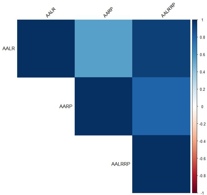 Figure 56: Correlation matrix plot
The correlation matrix presented by the Figure 56 shows the pairwise correlation coefficients between the variables: Automated Actuarial Loss Reserves (AALR), Automated Actuarial Risk Premiums (AARP), and Automated Actuarial Loss Reserves Risk Premiums (AALRRPs). The corrplot function visualizes these correlations with color coding. There is a strong positive correlation between AALR vs. AALRRP since AALR is a component of AALRRPs. A high correlation here confirms that the GPR model's predictions for loss reserves and their combination with risk premiums are consistent. There is also expected to show a high positive correlation between AARP vs. AALRRP, as AARP is another component of AALRRPs. A high correlation indicates that the GPR model is effectively capturing the relationship between risk premiums and the overall combined metric. While AALR and AARP are be related through the model's estimation process, their correlation is moderate compared to their relationships with AALRRPs. This indicates that the GPR model differentiates between the loss reserves and risk premiums in a meaningful way.
The high correlations between AALR and AALRRPs, and AARP and AALRRPs, support the idea that the GPR model is robust. It suggests that the model effectively captures how changes in loss reserves and risk premiums affect the combined metric (AALRRPs). Moderate or low correlation between AALR and AARP suggests that the model correctly estimates these components separately without overemphasizing their relationship, reflecting robustness in how it handles individual variables.
{"image_source":{"path":"images/c273956c29517753f842889ea257ef24c3a39c03b288647e953a0626e14e5d0e.jpg"},"content":"","chart_caption":[{"type":"text","content":"Figure 57: Scatter Plot of AALR vs AALRRPs"}],"chart_footnote":[]}
{"image_source":{"path":"images/8a9501c424d947c66fb3a06442e5ff87cbed0e7a8f538443c8f07565852cacc9.jpg"},"content":"","chart_caption":[{"type":"text","content":"Figure 58: Scatter Plot of AARP vs AALRRPs"}],"chart_footnote":[]}
The Figure 57 visualizes the relationship between Automated Actuarial Loss Reserves (AALR) and Automated Actuarial Loss Reserves Risk Premiums (AALRRPs). A positive trend in this scatter plot would indicate that as AALR increases, AALRRPs also increase, which is expected since AALR is part of the calculation for AALRRPs. The points generally align along a line or show a clear positive trend, it confirms that the GPR model's predictions for AALR are consistent with its predictions for AALRRPs. This linearity suggests the model's reliability in estimating AALRRPs based on AALR. There are no extreme outliers or clusters of points that deviate significantly, it indicates that the GPR model is stable and does not produce erratic or unrealistic predictions.
The Figure 58 visualizes the relationship between Automated Actuarial Risk Premiums (AARP) and Automated Actuarial Loss Reserves Risk Premiums (AALRRPs). A positive trend here indicates that as AARP increases, AALRRPs also increase. This is expected since AARP is another component of AALRRPs. A clear positive trend would support that the GPR model is robust, as it shows that changes in AARP are consistently reflected in changes in AALRRPs. Similar to the previous scatter plot, the absence of significant outliers suggests that the model produces stable and realistic predictions for risk premiums and their combination with loss reserves.
5.16.2. Stress Testing: Stress testing involves evaluating a model by subjecting it to extreme or adverse conditions to determine its breaking point or how it performs under significant pressure. This method is particularly important in fields like finance and insurance, where models must be resilient to extreme market conditions or catastrophic events , and .
{"image_source":{"path":"images/8e70143532a8d327c6edbbe11af28ce1896cc601977a64b71390ea12511fb8c4.jpg"},"content":"","chart_caption":[{"type":"text","content":"Figure 59: Stress Testing Plot"}],"chart_footnote":[]}
The Figure 59 displays a scatter plot of Automated Actuarial Loss Reserves Risk Premiums (AALRRPs) before and after applying a stress test where inflation is increased by . The plot includes a linear regression line to show the relationship between the original and stressed AALRRPs. The scatter plot shows a strong positive trend (points generally aligning with the diagonal line where Original AALRRPs equals Stressed AALRRPs), it indicates that the GPR model's estimates are consistent under the stress scenario. This positive relationship suggests that while the absolute values of AALRRPs have increased, the model's behavior is predictable and aligns well with the expected effect of the inflation increase. The red line represents the linear regression fit of the data points and a close alignment of this line with the diagonal suggests that the GPR model is robust, as the inflation stress test leads to a proportional increase in AALRRPs without introducing significant distortions.
In short, the stress test plot shows that the GPR model is robust because it provides consistent and reliable predictions even under stress scenarios. The proportional increase in AALRRPs with increased inflation and the absence of significant deviations or outliers indicate that the model effectively captures the relationships between the variables and responds predictably to changes
5.16.3. Scenario Testing: Scenario testing involves assessing a model's performance by simulating various hypothetical situations, each based on a different set of assumptions or conditions. Unlike stress testing, which focuses on extreme events, scenario testing considers a range of possible outcomes, including both positive and negative scenarios. This approach is often used to explore the potential impact of different future events or decisions on the model's outputs [40],[41] and [42].
{"image_source":{"path":"images/cba19c8bf3d3e6e0d34cb1b7ed18c1af811c296b1a52792be54dcd54057b2391.jpg"},"content":"","chart_caption":[{"type":"text","content":"Impact of Inflation Rates on Actuarial Estimates"},{"type":"text","content":"Figure 60: Scenario Testing plot"}],"chart_footnote":[]}
The Figure 60 produced from the scenario testing displays how changes in inflation rates impact the Automated Actuarial Loss Reserves, Risk Premiums, and the combined Loss Reserves Risk Premiums. The x-axis represents the inflation rate scenarios, ranging from 0.01 to 0.05 in increments of 0.01 and the y-axis represents the values of the actuarial estimates (Loss Reserves, Risk Premiums, and Total). The consistent horizontal trends in the Loss Reserves, Risk Premiums, and Total with increasing inflation rates demonstrate that the model responds logically and predictably to changes in inflation. This indicates that the model captures the impact of inflation effectively and provides a robust response to different inflation scenarios.
VI. DISCUSSION
The methodology proposed in this study introduces several key advancements in actuarial modeling for travel insurance. By leveraging Gaussian Process Regression (GPR), our approach captures complex non-linear relationships in claim data, leading to more precise predictions of claim frequency and severity compared to traditional parametric models. This non-parametric approach is particularly beneficial in handling the inherent variability and uncertainty in insurance data. The integration of an inflation adjustment model within the GPR framework enhances the model's ability to respond dynamically to economic changes, providing more accurate estimates of reserves and premiums. This is crucial for maintaining financial stability and regulatory compliance under IFRS 17. The application of advanced data visualization techniques, including clustering and dimensionality reduction, allows for a more granular analysis of policyholder data. The k-means clustering approach segments policyholders into distinct groups based on their actuarial profiles, facilitating targeted underwriting and risk management strategies. Visualization tools such as boxplots and density plots further enhance the understanding of data distributions and relationships, providing valuable insights for decision-making. Our robustness and stress testing procedures demonstrate the model's resilience to variations in inflation rates and other economic factors. The scenario analysis highlights the sensitivity of actuarial estimates to different inflation scenarios, offering a forward-looking perspective on potential risks and impacts. The inclusion of simulated actuarial features and expenses enriches the dataset, providing a more comprehensive evaluation of financial health. The recalculated IFRS 17 metrics, reflecting the impact of simulated expenses, offer a detailed assessment of financial performance and adherence to regulatory standards. In short, the proposed methodology represents a significant advancement in actuarial modeling for travel insurance. It combines sophisticated statistical techniques with a thorough understanding of regulatory requirements, offering a robust framework for pricing, underwriting, and financial reporting
VII. CONCLUSION
In conclusion, this study presents a comprehensive and innovative methodology for actuarial modeling and risk pricing in the travel insurance sector under IFRS 17. The use of Gaussian Process Regression (GPR) for predicting claim frequencies and severities, coupled with an inflation adjustment model, significantly enhances the accuracy and responsiveness of actuarial estimates. The integration of advanced clustering and visualization techniques provides valuable insights into policyholder data and supports more informed underwriting decisions. Our approach also includes rigorous testing and scenario analysis, which demonstrates the model's robustness and its ability to handle economic uncertainties. The simulated actuarial features and updated IFRS 17 metrics offer a detailed evaluation of financial health, contributing to improved regulatory compliance and financial reporting. The methodology introduced in this paper not only advances the field of actuarial science but also provides practical tools for better managing travel insurance risks. Future work could explore the application of these techniques to other lines of insurance or further refine the models based on real-world data. The continued development of such methodologies will be crucial for adapting to evolving regulatory standards and economic conditions in the insurance industry
7.1. Funding
The research was not supported by any funding.
7.2. Data availability
The data was simulated in R and kept for ethical reasons.
7.3. Declaration
There were no any conflicts of interest.
ACKNOWLEDGMENT
Special thanks goes to members of staff at University of Zimbabwe through the department of Mathematics & Computational sciences for both academic, social and moral support.
Conflict of Interest
The authors declare no conflict of interest.
Ethical Approval
Not applicable
Data Availability
The datasets used in this study are openly available at [repository link] and the source code is available on GitHub at [GitHub link].
Funding
This work did not receive any external funding.
References
Cite this article
Related Research


Special Issue
Launch a focused special issue to highlight research, emerging trends, and expert insights in your academic field.
