I. INTRODUCTION
Steganography can be comparable to protection of communication, as it is known as a technique being used in order to protect some information to be exchanged by hiding its original existence, onto some digital files, could it be a photographies or videograms. As we know of cryptography as the technique and science behind the protection of messages and information to be transmitted, the idea for steganography is actually to prevent a nasty observer to even detect the need for that protection firstly, and it is also depending on the situations, as for instance in places where cryptography cannot be used.
Sometimes, it is also possible to mix together both techniques for protection of communication and information. The classic example known to illustrate use of a steganographic scheme is the prisoners problem exchanging messages under the surveillance of a warden. Crandall was the first to suggest it and later Westfeld applied it.
The codes [2, 12, 13, 14] present an enrichment from the logical viewpoint and we can mathematically express that an information is lightly, partially or greatly damaged.
Let E be a finite set. A non-empty subset C of E is called a code. E is the set of n-tuples from a finite set with elements. Each element of E is called words and the elements of C, codewords. E is an n-dimensional vector space over , so .
Section 2 define firstly the modal -valent set structure and the algebra of , secondly the linear codes and lastly the Hamming -distance of . Section 3 presents the Hamming codes on . Section 4 is devoted to the steganographic protocol and Hamming codes.
II. PRELIMINARIES
2.1 The modal -valent set structure and the algebra of (FpZ; Fa)
Definition 0.1. [15] Let , be a chain whose first and last elements are 0 and 1 respectively, where .
A set is the pair or such that:
Theorem 0.1. [8]
Let be a set.
\[\forall x,y\in E,\,x=_\Theta y\iff\forall\alpha\in I_*,F_\alpha(x)=F_\alpha(y)\]
Proof 0.1. [8]
Definition 0.2. [12] Let . We call the set of invariant elements of the set .
Proposition 0.1. [8] Let be a set. The following properties are equivalent:
1.
-
-
;
-
.
Proof 0.2. [8]
Definition 0.3. [1]
Let and be two sets. We shall call
- a subset of if the structure of set is the restriction to of the structure of the set , that means:
- Let be a non-empty set. a subset of if:
Let be a prime number. Let us recall that if .
\[\mathbb {F} _ {p \mathbb {Z}} = \mathbb {F} _ {p} \cup \left\{x _ {p \mathbb {Z}}: \neg (x \equiv 0 (\text { mod } p)) \right\}; \quad \mathbb {F} _ {p} = \{0, 1, 2, \dots , p - 1 \}.\]
Let us define the support of as follows:
\[s \left(a\right) = \left\{ \begin{array}{l l} a & \text{if } a \in \mathbb{F}_{p}; \\ x & \text{if } a = x_{p \mathbb{Z}} \text{ with } \lceil (x \equiv 0 \pmod{p}). \end{array} \right.\]
Thus
Definition 0.4. [15] Let be a binary operation on . So, , . Let . We define a binary operation on as follows:
\[x \perp* y = \left\{
\begin{array}{l l}
s (x) \perp s (y) & \text{if } x, y \in \mathbb{F}_{p} \\
(s (x) \perp s (y)) \equiv 0 (\text{mod } p) & \text{otherwise} \\
(s (x) \perp s (y))_{p \mathbb{Z}} & \text{otherwise.}
\end{array}
\right.\]
as defined above on will be called a law on . So we can define and .
Theorem 0.2. [1] is a ring of unity 1 and of unity .
Proof 0.3. [1]
Remark 0.1. Since is prime, is a field.
Definition 0.5. [6] is a divisor of zero in if verifying
Example 0.1. [6] By this example, we show that , prime, is a field of elements.
, we have
The table of determination and tables laws of .
\mathbb{F}_{2\mathbb{Z}}
| $\mathbb{F}_{2\mathbb{Z}}$ | 0 | 1 | $1_{2\mathbb{Z}}$ | $3_{2\mathbb{Z}}$ |
| $F_1$ | 0 | 1 | 1 | 0 |
| $F_2$ | 0 | 1 | 0 | 1 |
| $+^{\Theta}$ | 0 | 1 | $1_{2\mathbb{Z}}$ | $3_{2\mathbb{Z}}$ |
| 0 | 0 | 1 | $1_{2\mathbb{Z}}$ | $3_{2\mathbb{Z}}$ |
| 1 | 1 | 0 | 0 | 0 |
| $1_{2\mathbb{Z}}$ | $1_{2\mathbb{Z}}$ | 0 | 0 | 0 |
| $3_{2\mathbb{Z}}$ | $3_{2\mathbb{Z}}$ | 0 | 0 | 0 |
\times^\Theta
| $\times^{\Theta}$ | 0 | 1 | $1_{2\mathbb{Z}}$ | $3_{2\mathbb{Z}}$ |
| 0 | 0 | 0 | 0 | 0 |
| 1 | 0 | 1 | $1_{2\mathbb{Z}}$ | $3_{2\mathbb{Z}}$ |
| $1_{2\mathbb{Z}}$ | 0 | $1_{2\mathbb{Z}}$ | $1_{2\mathbb{Z}}$ | $3_{2\mathbb{Z}}$ |
| $3_{2\mathbb{Z}}$ | 0 | $3_{2\mathbb{Z}}$ | $3_{2\mathbb{Z}}$ | $1_{2\mathbb{Z}}$ |
2.2 Linear m codes
Let be a finite set. , we will denote in what follows the set product of by ; where is the product on of . By definition, we have:
\[F _ {\alpha} ^ {n}: A ^ {n} \longrightarrow A ^ {n}; (a _ {1}, \dots , a _ {n}) \longmapsto F _ {\alpha} ^ {n} (a _ {1}, \dots , a _ {n}) = (F _ {\alpha} (a _ {1}), \dots , F _ {\alpha} (a _ {n}))\]
such that .
Definition 0.6. [14] Let us set the image of . As is injective, is a bijection from to . is considered as the set of all possible messages.
-
A code of length and of alphabet , the set .
-
Elements of , messages or words of the code .
-
Elements of , , messages or words of the code .
Proposition 0.2. [12] is a part of .
Proof 0.4. [12]
Proposition 0.3. [12] Let be a code of length on . The set is a classical code of length on .
Definition 0.7. [13] Let be the field with Card ,
- Hamming -weight of is the number , of non zero coordinates of .
\[\omega_ {H _ {\alpha}} (x) = \omega \left(F _ {\alpha} ^ {n} (x)\right) = \operatorname{Card} \left\{i \mid F _ {\alpha} \left(x _ {i}\right) \neq 0; i = 1, \dots , n \right\}.\] 2. Hamming -weight of is the number and defined by:
\[\omega_{H_{\Theta}}(x) = \left\{ \begin{array}{l l} \omega(x) & x \in \mathbb{F}_{2}^{n}; \\ \sum_{\alpha \in I_{*}} \omega_{H_{\alpha}}(x) = \sum_{\alpha \in I_{*}} \omega(F_{\alpha}^{n}(x)) & \text{otherwise}. \end{array} \right.\]
The alphabet used is the field .
Proposition 0.4. [6] We set and . Let be the set of message and a linear encoder of in . Then, the code is a vector subspace of over .
Proof 0.6. [6]
Definition 0.8. [14] A linear code of length and of dimension on is a vector subspace of of dimension .
Proposition 0.5. [6] Let be a linear code of length and of dimension .
Then is a linear code of length and of dimension .
Proof 0.7. [6] As is a -vector space of dimension , so is a linear code of length and .
2.3 The Hamming -distance of
Let be a or a pseudo code on of length n. In , let us define a notion compatible with the structure of code called distance.
on is defined by:
\[\begin{array}{r c l} {d _ {H _ {\alpha}} (x, y)} & = & {d _ {H} (F _ {\alpha} ^ {n} x, F _ {\alpha} ^ {n} y)} \\& = & {c a r d \{i: F _ {\alpha} x _ {i} \neq F _ {\alpha} y _ {i}; i = 1, \dots , n \}.} \end{array}\]
Where ; and is the Hamming distance on .
Proposition 0.6. If is a set and is a code on , then
on is defined by:
\[d_{H_{\Theta}}(x,y) = \left\{ \begin{array}{ll} d_H(x,y) & \text{if } x \text{ and } y \in (C(A,F_{\alpha}))^n; \\ \sum_{\alpha \in I_*} d_{H_\alpha}(x,y) = \sum_{\alpha \in I_*} d_H(F_\alpha x, F_\alpha y) & \text{otherwise.} \end{array} \right.\]
distance on
Proof 0.8. [12]
Definition 0.9. will be called the Hamming distance on .
Definition 0.10. Let be a code; is the Hamming distance. We define as follows:
\[\delta^\Theta = \min \left\{ d_{H_\Theta} (x, y) : x, y \in \mathcal{C}; x \neq y \right\}\]
is the minimal distance of the code .
III. THE HAMMING MΘ CODES
3.1 Dual mΘ codes
Let , , be a linear code in . Let G be a matrix whose rows generate . Let G be a generating matrix of .
The dual code of , denoted , is defined as follows
\[\mathcal{C}^\perp = \left\{x \in V(n, p\mathbb{Z}); \forall \alpha \in I_*, \langle F_\alpha x, F_\alpha c\rangle = 0, \forall c \in (\mathcal{C}, F_\alpha)\right\}\]
is clearly also a linear code, and has a generating matrix . By the definition of ,
\[\mathcal{C} = \{c \in V(n, p\mathbb{Z}) / \forall \alpha \in I_{*}, F_{\alpha}(c) H^{t} = 0\}.\]
Where H is a parity check matrix for . If a word u is received, then it can be verified that u is a codeword such that , i.e., .
3.2 Hamming Codes on V (n; 2Z)
Hamming code is a linear code in for some . Let be the field of four elements and let H be the matrix whose columns are all the non-zero vectors of length k over . Note that there will be of these. We define the Hamming code as follows:
Definition 0.11. Let and . Let H denote the matrix. The Hamming code, , is the linear subspace of consisting of the set of all -vectors, , orthogonal to all the rows of H.
\[Ham_{2\mathbb{Z}}(n) = \{v \in V(n, 2\mathbb{Z}) / \forall \alpha \in I_*, F_\alpha(v) \times H^t = 0\}.\]
Proposition 0.7. The Hamming code is a -code with parity check matrix.
Proof 0.9. [3]
IV. THE MΘ STEGANOGRAPHIC PROTOCOL F5 AND HAMMING MΘ CODES
4.1 The mΘ protocol F5
F5 is a steganographic system developed by Westfeld in 2001 [11]. The protocol F5 over permits to hide messages of length k in cover words of length by partially or totally changing more than one of them.
Let be the -binary word of m with k bits, . Conversely, for , , let be an element of which has as -binary word, so .
Lastly, let be the -vector of the canonical basis of ; .
Proposition 0.8. The maps , , and as follows define:
\[\gamma_{2\mathbb{Z}}: V(2^{k} - 1, 2\mathbb{Z}) \times V(k, 2\mathbb{Z}) \longrightarrow (\mathbb{N}_{2\mathbb{Z}}, F'_{\alpha})\]
\[(x, m) \longmapsto (< F _ {\alpha} ^ {k} (m) + \sum_ {i = 1} ^ {2 ^ {k} - 1} F _ {\alpha} (x _ {i}) < i > _ {2} > _ {10}) _ {\alpha \in I _ {*}}\]
\[\begin{array}{r c l} e _ {2 \mathbb {Z}}: V (2 ^ {k} - 1, 2 \mathbb {Z}) \times V (k, 2 \mathbb {Z}) & \longrightarrow & V (2 ^ {k} - 1, 2 \mathbb {Z}) \\(x, m) & \longmapsto & (F _ {\alpha} ^ {2 ^ {k} - 1} (u) + e _ {F _ {\alpha} ^ {\prime} (\gamma_ {2 \mathbb {Z}} (x, m))}) _ {\alpha \in I _ {*}} \end{array}\]
\[r_{2\mathbb{Z}}: V(2^{k} - 1, 2\mathbb{Z}) \longrightarrow V(k, 2\mathbb{Z})\]
\[x \longmapsto (\sum_ {i = 1} ^ {2 ^ {k} - 1} F _ {\alpha} (x _ {i}) < i > _ {2}) _ {\alpha \in I _ {*}}\]
are well defined and .
Proof 0.10.
\[(i) \quad \bullet L e t (x, m), (x ^ {\prime}, m ^ {\prime}) \in V (2 ^ {k} - 1, 2 \mathbb {Z}) \times V (k, 2 \mathbb {Z})\]
let us suppose that ( and ) and let us show that .
\[(x, m) = (x ^ {\prime}, m ^ {\prime}) \implies \forall \alpha \in I _ {*} \left\{ \begin{array}{l} F _ {\alpha} ^ {2 ^ {k} - 1} x = F _ {\alpha} ^ {2 ^ {k} - 1} x ^ {\prime} \\ F _ {\alpha} ^ {k} m = F _ {\alpha} ^ {k} m ^ {\prime} \end{array} \right.\]
\[\begin{array}{l} F _ {\alpha} ^ {k} m + \sum_ {i = 1} ^ {2 ^ {k} - 1} F _ {\alpha} x _ {i} < i > _ {2} = F _ {\alpha} ^ {k} t + \sum_ {i = 1} ^ {2 ^ {k} - 1} F _ {\alpha} x _ {i} ^ {\prime} < i > _ {2} \\\Longrightarrow < F _ {\alpha} ^ {k} m + \sum_ {i = 1} ^ {2 ^ {k} - 1} F _ {\alpha} x _ {i} < i > _ {2} > _ {1 0} = < F _ {\alpha} ^ {k} m ^ {\prime} + \sum_ {i = 1} ^ {2 ^ {k} - 1} F _ {\alpha} x _ {i} ^ {\prime} < i > _ {2} > _ {1 0} \\\Longrightarrow (< F _ {\alpha} ^ {k} m + \sum_ {i = 1} ^ {2 ^ {k} - 1} F _ {\alpha} x _ {i} < i > _ {2} > _ {1 0}) _ {\alpha \in I _ {*}} = (< F _ {\alpha} ^ {k} m ^ {\prime} + \sum_ {i = 1} ^ {2 ^ {k} - 1} F _ {\alpha} x _ {i} ^ {\prime} < i > _ {2} > _ {1 0}) _ {\alpha \in I _ {*}} \\\Longrightarrow \gamma_ {2 \mathbb{Z}} (x, m) = \gamma_ {2 \mathbb{Z}} (x ^ {\prime}, t) \end{array}\]
Therefore the map is well defined.
Let ,
\[\gamma_{2\mathbb{Z}} \circ (F_{\alpha}^{2^k-1}, F_{\alpha}^k)(x, m) = \gamma_{2\mathbb{Z}}(F_{\alpha}^{2^k-1} x, F_{\alpha}^k m)\]
\[\begin{array}{r c l} F _ {\alpha} ^ {\prime} \circ \gamma_ {2 \mathbb {Z}} (x, m) & = & F _ {\alpha} ^ {\prime} (< F _ {\alpha} ^ {k} m + \sum_ {i = 1} ^ {2 ^ {k - 1}} F _ {\alpha} x _ {i} < i > _ {2} > _ {1 0}) _ {\alpha \in I _ {*}} \\& = & (< F _ {\alpha} ^ {k} m + \sum_ {i = 1} ^ {2 ^ {k} - 1} F _ {\alpha} x _ {i} < i > _ {2} > _ {1 0}) _ {\alpha \in I _ {*}} \end{array}\]
Therefore is a map.
(ii)
- , such that ( and ), let's show that .
\[(x, m) = (x ^ {\prime}, m ^ {\prime}) \Longrightarrow \forall \alpha \in I _ {*}, \left\{ \begin{array}{l} F _ {\alpha} ^ {2 ^ {k} - 1} x = F _ {\alpha} ^ {2 ^ {k} - 1} x ^ {\prime} \\ F _ {\alpha} ^ {k} m = F _ {\alpha} ^ {k} m ^ {\prime} \end{array} \right.\]
\[\begin{array}{rl}
\forall \alpha \in I _ {*}, & \left\{
\begin{array}{l}
F _ {\alpha} ^ {2 ^ {k} - 1} x = F _ {\alpha} ^ {2 ^ {k} - 1} x ^ {\prime} \\
F _ {\alpha} ^ {k} m = F _ {\alpha} ^ {k} m ^ {\prime}
\end{array}
\right.
\Rightarrow \forall \alpha \in I _ {*}, \left\{
\begin{array}{l}
F _ {\alpha} ^ {2 ^ {k} - 1} x = F _ {\alpha} ^ {2 ^ {k} - 1} x ^ {\prime} \\
\gamma_ {2 \mathbb {Z}} (x, m) = \gamma_ {2 \mathbb {Z}} (x ^ {\prime}, m ^ {\prime})
\end{array}
\right. \\
& \Rightarrow \forall \alpha \in I _ {*}, \left\{
\begin{array}{l}
F _ {\alpha} ^ {2 ^ {k} - 1} x = F _ {\alpha} ^ {2 ^ {k} - 1} x ^ {\prime} \\
F _ {\alpha} ^ {\prime} \gamma_ {2 \mathbb {Z}} (x, m) = F _ {\alpha} ^ {\prime} \gamma_ {2 \mathbb {Z}} (x ^ {\prime}, m ^ {\prime})
\end{array}
\right. \\
& \Rightarrow \forall \alpha \in I _ {*}, \left\{
\begin{array}{l}
F _ {\alpha} ^ {2 ^ {k} - 1} x = F _ {\alpha} ^ {2 ^ {k} - 1} x ^ {\prime} \\
e _ {F _ {\alpha} ^ {\prime} \gamma_ {2 \mathbb {Z}} (x, m)} = e _ {F _ {\alpha} ^ {\prime} \gamma_ {2 \mathbb {Z}} (x ^ {\prime}, m ^ {\prime})}
\end{array}
\right. \\
\Rightarrow & \forall \alpha \in I _ {*}; F _ {\alpha} ^ {2 ^ {k} - 1} x + e _ {F _ {\alpha} ^ {\prime} \gamma_ {2 \mathbb {Z}} (x, m)} = F _ {\alpha} ^ {2 ^ {k} - 1} x ^ {\prime} + e _ {F _ {\alpha} ^ {\prime} \gamma_ {2 \mathbb {Z}} (x ^ {\prime}, m ^{\prime})} \\
\Rightarrow & (F _ {\alpha} ^ {2 ^ {k} - 1} x + e _ {F _ {\alpha} ^ {\prime} \gamma_ {2 \mathbb {Z}} (x, m)} = F _ {\alpha} ^ {2 ^ {k} - 1} x ^ {\prime} + e _ {F _ {\alpha} ^ {\prime} \gamma_ {2 \mathbb {Z}} (x ^ {\prime}, m ^{\prime})}) _ {\alpha \in I _ {*}} \\
& \Rightarrow e _ {2 \mathbb {Z}} (x, m) = e _ {2 \mathbb {Z}} (x ^ {\prime}, m ^ {\prime}).
\end{array}\]
Therefore is well defined.
\[\begin{array}{r c l} L e t (x, m) \in V (2 ^ {k} - 1, 2 \mathbb {Z}) \times V (k, 2 \mathbb {Z}) \\e _ {2 \mathbb {Z}} \circ (F _ {\alpha} ^ {2 ^ {k} - 1}, F _ {\alpha} ^ {k}) (x, m) & = & e _ {2 \mathbb {Z}} (F _ {\alpha} ^ {2 ^ {k} - 1} x, F _ {\alpha} ^ {k} m) \\& = & (F _ {\alpha} ^ {2 ^ {k} - 1} (F _ {\alpha} ^ {2 ^ {k} - 1} x) + e _ {F _ {\alpha} ^ {\prime} \gamma_ {2 \mathbb {Z}} (F _ {\alpha} ^ {2 ^ {k} - 1} x, F _ {\alpha} ^ {k} m)}) _ {\alpha \in I _ {*}} \\& = & (F _ {\alpha} ^ {2 ^ {k} - 1} x + e _ {F _ {\alpha} ^ {\prime} \gamma_ {2 \mathbb {Z}} (x, m)}) _ {\alpha \in I _ {*}} (\gamma_ {2 \mathbb {Z}} i s m \Theta m a p). \\F _ {\alpha} ^ {\prime} \circ e _ {2 \mathbb {Z}} (x, m) & = & F _ {\alpha} ^ {\prime} (F _ {\alpha} ^ {2 ^ {k} - 1} x + e _ {F _ {\alpha} ^ {\prime} (\gamma_ {2 \mathbb {Z}} (x, m))}) _ {\alpha \in I _ {*}} \\& = & (F _ {\alpha} ^ {2 ^ {k} - 1} x + e _ {F _ {\alpha} ^ {\prime} (\gamma_ {2 \mathbb {Z}} (x, m))}) _ {\alpha \in I _ {*}}. \end{array}\]
Therefore;
\[e _ {2 \mathbb {Z}} \circ (F _ {\alpha} ^ {2 ^ {k} - 1}, F _ {\alpha} ^ {k}) = F _ {\alpha} ^ {\prime} \circ e _ {2 \mathbb {Z}}.\]
(iii) Let us show that is well defined.
Let us suppose that ( ) and let us show that .
Let ;
\[F_{\alpha}^{2^{k}-1}(x) = F_{\alpha}^{2^{k}-1}(x^{’}) \Rightarrow F_{\alpha} x_{i} = F_{\alpha} x_{i}^{’} \Rightarrow F_{\alpha} x_{i} < i >_{2} = F_{\alpha} y_{i} < i >_{2} \Rightarrow \sum_{i=1}^{2^{k}-1} F_{\alpha} x_{i} < i >_{2} = \sum_{i=1}^{2^{k}-1} F_{\alpha} x_{i}^{’} < i >_{2} \Rightarrow (\sum_{i=1}^{2^{k}-1} F_{\alpha} x_{i} < i >_{2})_{\alpha \in I_{*}} = (\sum_{i=1}^{2^{k}-1} F_{\alpha} x_{i}^{’} < i >_{2})_{\alpha \in I_{*}} \Rightarrow r_{2\mathbb{Z}}(x) = r_{2\mathbb{Z}}(x^{’})\]
Therefore is a map.
Let , let .
\[\begin{array}{r c l} r _ {2 \mathbb {Z}} \circ F _ {\alpha} ^ {2 ^ {k} - 1} (x) & = & r _ {2 \mathbb {Z}} (F _ {\alpha} ^ {2 ^ {k} - 1} x) \\& = & (\sum_ {i = 1} ^ {2 ^ {k} - 1} F _ {\alpha} ((F _ {\alpha} ^ {2 ^ {k} - 1} x) _ {i}) < i > _ {2}) _ {\alpha \in I _ {*}} \\& = & (\sum_ {i = 1} ^ {2 ^ {k} - 1} F _ {\alpha} (F _ {\alpha} x _ {i}) < i > _ {2}) _ {\alpha \in I _ {*}} \\& = & (\sum_ {i = 1} ^ {2 ^ {k} - 1} F _ {\alpha} x _ {i} < i > _ {2}) _ {\alpha \in I _ {*}} \end{array}\]
\[F_{\alpha}^{\prime} \circ r_{2\mathbb{Z}}(x,m) = F_{\alpha}^\prime ( (\sum_{i=1}^{2^{k}-1} F_{\alpha} x_{i} < i > _{2})_{\alpha \in I_{*}} ) \\= (\sum_{i=1}^{2^{k}-1} F_{\alpha} x_{i} < i > _{2})_{\alpha \in I_{*}}\]
Therefore is a map.
Proposition 0.9. before define in the proposition 0.8 is a steganographic protocols.
Proof 0.11. Let's show that is a steganographic protocol. In other words, , for any and for any .
\[So, \forall\alpha\in I_*, F_{\alpha}^k(r_{2\mathbb{Z}}(e_{2\mathbb{Z}}(x,m))) = F_{\alpha}^k(m)\]
1.
\[F_{\alpha}^{k}(r_{2\mathbb{Z}}(e_{2\mathbb{Z}}(x,m))) = r_{2\mathbb{Z}}(F_{\alpha}^{2^{k}-1} \circ e_{2\mathbb{Z}}(x,m)) (r_{2\mathbb{Z}} is m\Theta map) = r_{2\mathbb{Z}}(e_{2\mathbb{Z}} \circ (F_{\alpha}^{2^{k}-1}, F_{\alpha}^{k}))(x,m) (e_{2\mathbb{Z}} is a m\Theta map) = r_{2\mathbb{Z}}(e_{2\mathbb{Z}}(F_{\alpha}^{2^{k}-1} x, F_{\alpha}^{k} m)) = r_{2\mathbb{Z}}(F_{\alpha}^{2^{k}-1} x + e_{F_{\alpha}'(\gamma_{2\mathbb{Z}}(x,m))}).\]
we put
\[j = F_{\alpha}^{\prime}(\gamma_{2\mathbb{Z}}(x, m)) = \gamma_{2\mathbb{Z}} \circ (F_{\alpha}^{2^k - 1}, F_{\alpha}^k)(x, m) = \gamma_{2\mathbb{Z}}(F_{\alpha}^{2^k - 1} x, F_{\alpha}^k m) = < F_{\alpha}^k (F_{\alpha}^k m) + \sum_{i=1}^{2^k - 1} F_{\alpha}((F_{\alpha}^{2^k - 1} x)_i) < i >_2 >_{10} = < F_{\alpha}^k m + \sum_{i=1}^{2^k - 1} F_{\alpha}(F_{\alpha} x_i) < i >_2 >_{10} = < F_{\alpha}^k m + \sum_{i=1}^{2^k - 1} F_{\alpha}(x_i) < i >_2 >_{10}\]
\[then < j >_2 = F_{\alpha}^k m + \sum_{i=1}^{2^k - 1} F_{\alpha}(x) < i >_2\]
2.
\[r_{2\mathbb{Z}}(F_{\alpha}^{2^k-1} x + e_j) = r_{2\mathbb{Z}}(F_{\alpha} x_1, F_{\alpha} x_2, \dots , F_{\alpha} x_j + 1, \dots , F_{\alpha} x_n) \\= \sum_{i=1,i\neq j}^{2^k-1} \{F_{\alpha}(F_{\alpha} x_i) < i >_2 + (F_{\alpha} x_j + 1) < j >_2\} \\= \sum_{i=1,i\neq j}^{2^k-1} \{F_{\alpha}(x_i) < i >_2 + (F_{\alpha} x_j + 1) < j >_2\}\]
changing by expression given in (*) we get:
\[\forall \alpha \in I _ {*}, F _ {\alpha} ^ {k} (r _ {2 \mathbb {Z}} (e _ {2 \mathbb {Z}} (x, m))) = F _ {\alpha} ^ {k} (x, m).\]
Therefore, . Thus protocol F5 is a steganographic protocol.
Remark 0.2.
-
Embed a message s by the steganographic protocol F5 in a cover u consists to swap the coordinate number .
-
extraction consists to add all products of each -component, , to the value of the expression of the index. In other words,
\[r_{2\mathbb{Z}}(u) = \sum_{i=1}^{2^k-1} F_{\alpha} u_i < i >_2.\]
Example 0.2. Let be a Hamming code, k = 3. We want to insert into by the steganographic protocol F5.
, , , .
So, how to calculate .
\[\gamma_{2\mathbb{Z}}(1_{2\mathbb{Z}}1_{2\mathbb{Z}}003_{2\mathbb{Z}}01_{2\mathbb{Z}}, 01_{2\mathbb{Z}}1_{2\mathbb{Z}}) = (< F_{1}^{3}(01_{2\mathbb{Z}}1_{2\mathbb{Z}}) + \sum_{i=1}^{7} F_{1}x_{i} < i >_{2}>_{10},< F_{2}^{3}(01_{2\mathbb{Z}}1_{2\mathbb{Z}}) + \sum_{i=1}^{7} F_{2}x_{i} < i >_{2}>_{10})\]
\[\begin{array}{r c l} < F _ {1} ^ {3} (0 1 _ {2 \mathbb {Z}} 1 _ {2 \mathbb {Z}}) + \sum_ {i = 1} ^ {7} F _ {1} x _ {i} < i > _ {2} > _ {1 0} & = & < 0 1 1 + 1 (0 0 1) + 1 (0 1 0) + 1 (1 1 1) > _ {1 0} \\& = & 7 \end{array}\]
and
\[\begin{array}{r c l} < F _ {2} ^ {3} (0 1 _ {2 \mathbb {Z}} 1 _ {2 \mathbb {Z}}) + \sum_ {i = 1} ^ {7} F _ {2} x _ {i} < i > _ {2} > _ {1 0} & = & < 0 0 0 + 1 (1 0 1) > _ {1 0} \\& = & 5. \end{array}\]
\[\gamma_ {2 \mathbb {Z}} (x, m) = (7; 5) = (F _ {1} ^ {\prime} (\gamma_ {2 \mathbb {Z}} (x, m)); F _ {2} ^ {\prime} (\gamma_ {2 \mathbb {Z}} (x, m))).\]
\[e_{2\mathbb{Z}}(x, m) = (F_1^7 x + e_{F'_1}(\gamma_{2\mathbb{Z}}(x, m)); F_2^7 x + e_{F'_2}(\gamma_{2\mathbb{Z}}(x, m)))\]
\[F _ {1} ^ {7} x + e _ {F _ {1} ^ {\prime} (\gamma_ {2 \mathbb {Z}} (x, m))} = 1 1 0 0 0 0 1 + e _ {7} = 1 1 0 0 0 0 1 + 0 0 0 0 0 0 1 = 1 1 0 0 0 0 0.\]
\[F_{2}^{7} x + e_{F_{2}^{\\'}}(\gamma_{2\mathbb{Z}}(x,m)) = 0000100 + e_{5} = 0000100 + 0000100 = 0000000.\]
\[\begin{array}{r c l} e _ {2 \mathbb {Z}} (x, m) & = & (1 1 0 0 0 0 0, 0 0 0 0 0 0 0) \\& = & 1 _ {2 \mathbb {Z}} 1 _ {2 \mathbb {Z}} 0 0 0 0 0 \\& = & v. \end{array}\]
Now, we will extract the message hidden in the stego-word .
In other words, how to calculate ? By definition of given in the remark 0.3.:
\[r_{2\mathbb{Z}}(y) = (\sum_{i=1}^{7} F_1 y_i < i >_2, \sum_{i=1}^{7} F_2 y_i < i >_2)\]
\[\begin{array}{r c l} r _ {2 \mathbb {Z}} (y) & = & (1 (0 0 1) + 1 (0 1 0); 1 (0 0 0)) \\& = & (0 1 1; 0 0 0) \\& = & 0 1 _ {2 \mathbb {Z}} 1 _ {2 \mathbb {Z}} \\& = & m. \end{array}\]
4.2 The F5 mΘ Algorithm
To increase embedding efficiency, the F5 algorithm introduces for the first time the concept of matrix embedding technique for embedding in the context of using Hamming codes.
More formally, the desired purpose of the matrix embedding technique is to communicate a message through the cover vector , modifying it as little as possible.
The principle is to change the cover vector x to stego vector y, such that:
\[H(F_{\alpha}y)_{\alpha\in I_*} = (F_{\alpha}m)_{\alpha\in I_*},\]
with the parity check matrix of Hamming code. The transformation of the cover vector x into y is then carried out by seeking the vector of modification :
\[(F_{\alpha} y)_{\alpha \in I_*} = (F_{\alpha}(x + e))_{\alpha \in I_*};\]
\[H(F_{\alpha}(x+e))_{\alpha\in I_*} = (F_{\alpha}m)_{\alpha\in I_*} \Longleftrightarrow H(F_{\alpha}e)_{\alpha\in I_*} = (F_{\alpha}m)_{\alpha\in I_*} - H(F_{\alpha}x)_{\alpha\in I_*}.\]
Example 0.3. Taking [7, 4] Hamming code, we explain how to embed 3 bits of into 7 pixels. Let be the message that we want to insert in the cover vector . The parity check matrix is therefore in the following form:
\[H = \left( \begin{array}{c c c c c c c} 0 & 0 & 0 & 1 & 1 & 1 & 1 \\0 & 1 & 1 & 0 & 0 & 1 & 1 \\1 & 0 & 1 & 0 & 1 & 0 & 1 \end{array} \right).\]
The purpose is to find the -vector such that .
Otherwise,
\[\left\{ \begin{array}{l} F _ {1} (m) = 0 1 1, \quad F _ {2} (m) = 0 0 0. \\ F _ {1} (x) = 1 1 0 0 0 0 1, \quad F _ {2} (x) = 0 0 0 0 1 0 1. \end{array} \right\}\]
So,
\[\begin{array}{l l} F _ {1} (m) - H \times F _ {1} (x) & = \left( \begin{array}{c} 0 \\1 \\1 \end{array} \right) - \left( \begin{array}{c c c c c c c} 0 & 0 & 0 & 1 & 1 & 1 & 1 \\0 & 1 & 1 & 0 & 0 & 1 & 1 \\1 & 0 & 1 & 0 & 1 & 0 & 1 \end{array} \right) \times \left( \begin{array}{c} 1 \\1 \\0 \\0 \\0 \\0 \\1 \end{array} \right) \\& = \left( \begin{array}{c} 0 \\1 \\1 \end{array} \right) - \left( \begin{array}{c} 1 \\0 \\0 \end{array} \right) \\& = \left( \begin{array}{c} 1 \\1 \\1 \end{array} \right). \end{array}\]
Thus, the modification -vector is .
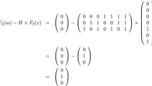
\[F_{2}(m) - H \times F_{2}(x) = \left( \begin{array}{l} 0 \\0 \\0 \end{array} \right) - \left( \begin{array}{lllllll} 0 & 0 & 0 & 1 & 1 & 1 & 1 \\0 & 1 & 1 & 0 & 0 & 1 & 1 \\1 & 0 & 1 & 0 & 1 & 0 & 1 \end{array} \right) \times \left( \begin{array}{l} 0 \\0 \\0 \\0 \\1 \\0 \\1 \end{array} \right) \\& = & \left( \begin{array}{l} 0 \\0 \\0 \end{array} \right) - \left( \begin{array}{l} 0 \\1 \\0 \end{array} \right) \\& = & \left( \begin{array}{l} 0 \\1 \\0 \end{array} \right).\]
Thus, .
\[e = (F_{1}(e), F_{2}(e)) = (0, 3_{2\mathbb{Z}}, 0, 0, 0, 0, 1_{2\mathbb{Z}}).\]
The cover vector x is then transformed into
\[\begin{array}{r c l} y = x + e & = & 1 _ {2 \mathbb {Z}} 1 _ {2 \mathbb {Z}} 0 0 3 _ {2 \mathbb {Z}} 0 1 _ {2 \mathbb {Z}} + 0 3 _ {2 \mathbb {Z}} 0 0 0 0 1 _ {2 \mathbb {Z}} \\& = & 1 _ {2 \mathbb {Z}} 0 0 0 3 _ {2 \mathbb {Z}} 0 0 \end{array}\]
We have the cover vector and the stego vector . When embedding m into x, it appears that 2 pixels of x have been partially damaged, namely the second and the last component of x. Indeed,
\[\left\{ \begin{array}{l} 1_{2\mathbb{Z}} = (F_{\alpha}1_{2\mathbb{Z}})_{\alpha\in I_*} = (F_11_{2\mathbb{Z}}, F_21_{2\mathbb{Z}}) = (1, 0) \\ 0 = (F_{\alpha}0)_{\alpha\in I_*} = (F_10, F_20) = (0, 0) \end{array} \right.\]
The passage from to 0 shows that the pixels has been partially damaged.
V. CONCLUSION
This note shows that the Hamming code is a -vector subspace of of dimension n. It appears that there exists a close relation between the protocols F5 and the Hamming code. The embedding of a message of k bits into the cover vector of n pixels changes at the level of the -modalities because it partially or totally damages at most one pixel of the cover vector.