this is test paper 2

# I. INTRODUCTION Testing, inspection, and certification (TIC) techniques play a crucial role in developing effective material modification treatments, [1], [2], [3], [4], [5], [6], [7], [8], [9], [10]. These methods cover a wide range of evaluations, such as fatigue, impact, composition, shear, thermomechanical, or liquid flow testing, that are essential for ensuring the performance and safety of modern composite materials. Modern structures, such as aerospace components, rehabilitation devices, and vehicle parts, often consist of heterogeneous, anisotropic composites (e.g., metals, carbon fiber, resins, and thermoplastics), which present unique challenges in terms of detection and evaluation to maintain structural integrity. A variety of destructive and non-destructive testing (DT/NDT) methods have been developed for these materials. Techniques include visual testing [8], thermographic testing, and several ultrasonic methods (Pulse Echo, Phased Array, and Thru-transmission) [2], [9], [10], [11], all designed to locate defects in single and multi-layer materials. Shearography [12] detects flaws in solid laminates and bonded surfaces through interferometric imaging under stressed and unstressed conditions. Other techniques, such as magnetic particle, liquid penetrant, optical, and eddy current testing (ECT) [13], are used to identify defects on and beneath surfaces in conductive materials. Radiographic testing, encompassing both 2D X-ray inspection and 3D computed tomography (CT) [2], [3], [4], [11], [12], [13], [14], [15] further enhances the ability to detect internal density variations indicative of flaws. Moreover, advanced synchrotron techniques using free electron lasers have begun to overcome some X-ray penetration limitations, producing intense and tunable beams for superior resolution [4], [7], [16], [17], [18], [19]. Despite these advances, all these methods share several limitations and unresolved challenges. Processing and analyzing data remain time-consuming and requires considerable expertise, particularly when overlapping signal amplitudes make it difficult to associate them with specific damage mechanisms. Many tools employ small gantries, limiting their field of view (FoV) and hindering their application on large, non-axisymmetric structures. Surface and shallow scanning techniques often face occlusion issues, rendering deep scanning in multilayered and complex geometries unreliable. Signal noise and diffractive scattering from grain and pore boundaries further complicate image analysis. Techniques like wet magnetic particle testing rely heavily on subjective visual feedback, while assumptions in ultrasonic testing regarding constant reflection coefficients can lead to inaccuracies [2], [9], [10], [11], [12]. Additional imaging challenges include issues with figure-to-ground relationships, background luminance, line dimensions, viewing distance, orientation, frequency-dependent attenuation, spatial resolution, contrast, density, radiographic mottle, distortion, metal artifacts, and non-linear signal responses—all of which can affect the detection of subsurface discontinuities, recrystallization states, and grain sizes [9], [10], [11], [12], [13], [14], [15], [16], [17], [18], [19]. Traditional industrial CT scanners are also limited by their relatively small or inflexible gantries, their inability to dynamically adjust the focal spot, and their lack of automatic control over image magnification related to amplitude and exposure. These scanners typically require the target to be motionless, and even state-of-the-art micro- and nanotomography systems, which are confined to very small gantries, can only be used on extensively prepared, in-situ small samples, thereby limiting their application for on-site inspections. A major common challenge is the motion artifact (blurriness) that occurs when inspecting moving objects. Direct measurement of internal kinematics, strain, and shear under high-speed motion has proven elusive. Although some studies have employed texture-mapped 2D models or manually segmented geometric models with template matching [14], [19], [20], [21], [22], [23], [24], [25], these approaches lack the accuracy required for comprehensive kinematics analysis, particularly in the presence of soft tissue or composite structures with variable material distribution. While 3D techniques like CT and magnetic resonance imaging (MRI) allow for direct observation of underlying structures, they do not yet achieve the high frame rates necessary for dynamic function estimation, and their confined imaging environments hinder full-motion kinematics measurement. Furthermore, none of these techniques has been standardized to date in terms of homologating dynamic inspection methods into a unified framework. There is a need to integrate these methods under a common reference system, both in terms of coordinate systems for data expression and normalization of kinematics data obtained from both marker-based and markerless tracking. All the above conventional testing techniques can last from several hours, to days or even months, as in the case of Maintenance, Repair, and Overhaul (MRO) A, B, C, D airplane checks [23], [26], depending on the size and complexity of the target and the laborious task of disassembling its parts to scan in the laboratory. The proposed robotics-driven multimodal imaging system with real-time motion compensation uniquely addresses these longstanding limitations. Unlike traditional systems, this platform is designed to inspect moving objects by dynamically compensating for motion artifacts, ensuring high-resolution imaging even during operation. Moreover, by unifying multiple imaging modalities under a The proposed robotics-driven multimodal imaging system with real-time motion compensation uniquely addresses these longstanding limitations. Unlike traditional systems, this platform is designed to inspect moving objects by dynamically compensating for motion artifacts, ensuring high-resolution imaging even during operation. Moreover, by unifying multiple imaging modalities under a common reference system, our system bridges the gap between disparate inspection methods, eliminating data inconsistencies and errors. This comprehensive approach not only enhances the detection of defects and internal anomalies in composite materials but also paves the way for more accurate and efficient on-site inspections across a variety of engineering fields. # II. 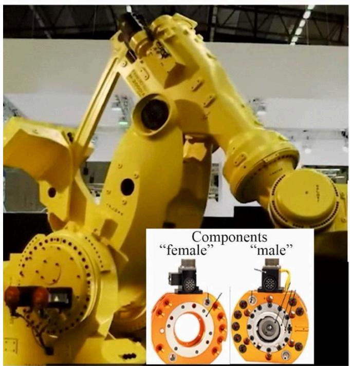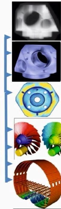METHODS # 2.1 System Overview and Data Acquisition The research leading to current state of the art of the device presented here can be summarized in the following references: [6], [14], [27], [28], [29], [30], [31], [32], [33], [34]. The Logimagine Helios System (KINEMAGINE/ATLAS Inc., [35]) used here employs several six to twelve-axis coordinated robotic systems. Configurations range from two to six robots (or cobots), programmed to carry combinations of X-ray housing units, dynamic flat panels, multicamera vision systems, intensifiers with high-speed radiography cameras, and densitometry detectors (fig. 1). The figure 1 presents the "One device-multiple modalities" principle and data fusion in the robotic scanner where the large robotic arm tool (far left) connects the end-of-arm tool (EoAT) with several multifunctionality connectors with a "female" component. Many male components of the device are attached to different detectors and emitters. These include intensifiers with high-speed X-Ray cameras, flat panels of different properties, large DEXA panels, perovskites panels, scintillation panels, different emitter and collimator combinations etc. This in turn, enables scanning an object in the same field of view with different emitter-detector combinations i.e., scan it with multiple modalities. These modalities (1-8) are digital radiography (DR), Panoramic and 360 DR, high-definition Micro CT, CT, 2D and 3D high speed stereovideoradiography with two (or more) planes, 2D and 3D tomosynthesis (Tomosynthesis, is a modality similar to, but distinct from CT which uses a more limited angle in image acquisition. Rather than a 360-degree acquisition of a structure, tomosynthesis, via an x-ray tube 'arcing' method over a stationary detector, can capture an arc sweep of a single part of the structure [28], [30], [32], [36]. This technique reduces the burden of overlapping structures/composites when assessing for single entities such as composite materials and layered objects. One of the primary advantages of tomosynthesis is its very high-resolution capabilities (as it functions as a magnification method); Tomosynthesis, if combined with optical magnification it can reach $10\mu \mathrm{m}$ resolution. The far-right column of images in figure 1 shows different types of imaging of various size objects (machine parts, jet turbines fuselage support structure etc.) that resulted from the aforementioned modalities.  Figure 1: Robotic scanner architecture illustrating the "One Device-Multiple Modalities" principle, where coordinated robotic arms integrate various emitter-detector combinations (e.g., DR, CT, tomosynthesis, stereovideoradiography) to capture multimodal images in a single field of view.     Several robots of different additional robotic arm types can be utilized interchangeably in the device. The system is manipulated via a computer and a human machine interface (HMI) device that stores a plethora of TIC imaging protocols. End-of-arm toolkits at the robots can exchange different emitters and detectors therefore employing different imaging modalities in the same calibration space. A collection of rails, pedestals and mobile trailers can extend the system's functional scanning envelop to reach targets up to 160 feet tall and of "unlimited" width and breadth (fig. 1, 2).       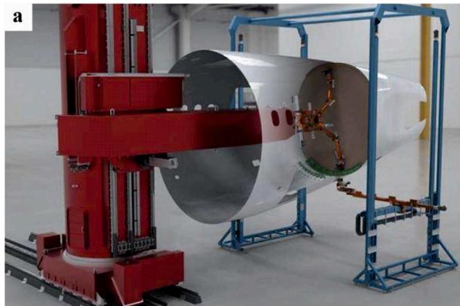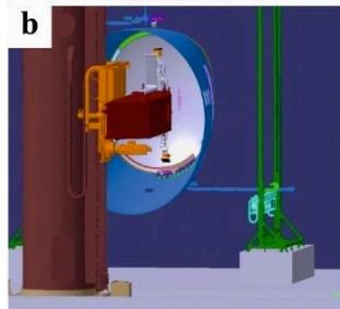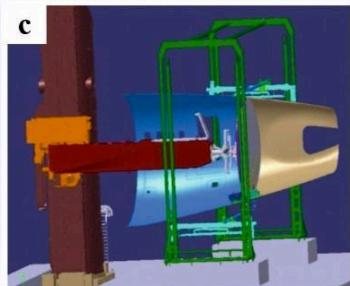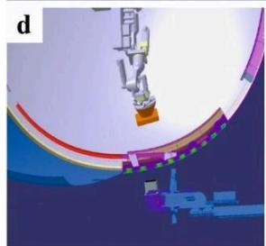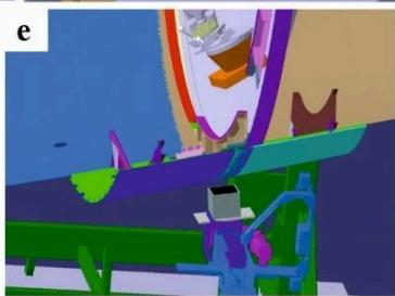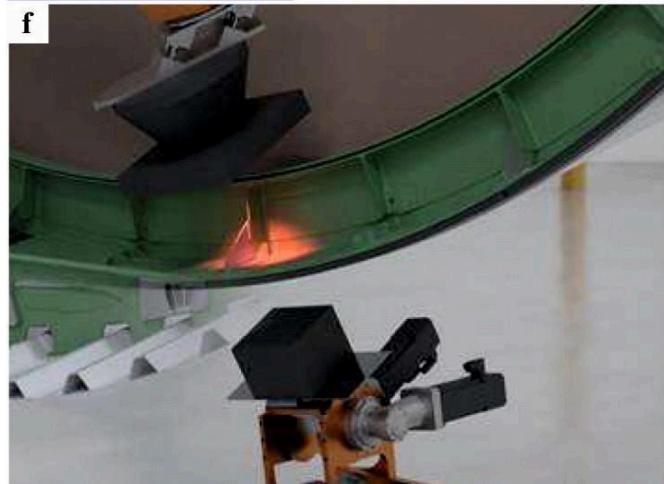Figure 2: (a) Large size robotic scanner mobilized by a huge base on a rail system with multiple degrees of freedom to approach the inside of a plane fuselage (with 160 feet high and up to 120 foot reach capacity so it can approach the full length of large long and non-axisymmetric objects (plane wings, jet engines, fuselages, large vehicle components, pipes etc.); (b)-(e) show the leading scanning robots carrying emitters and detectors as they approach the part in the fuselage to actually scan i.e., a deep layered joint of the connection of the cockpit to the fuselage as shown in (f). The "one-system-many-(potential) modalities" options ensure error free fusion of all the imaging modalities and co-registration of all the data in one unique robotic coordinate system (fig. 3), [27], [31], [32], [33], [34], [37], [38]. The last large-scale imaging modality for huge structures is very important as the scanning logistics with large objects that normally do not fit in the gantries of traditional scanners can be extremely laborious and most of the times impossible. These modalities can be tuned to provide industrial CT and microCT damage inspection, porosity analysis, dimensionality analysis, failure analysis, reverse engineering, 2D radiography with panoramic large format and automatically stitched imaging for huge and non-axisymmetric objects, densitometry of composites and stereofluoroscopy in 3D. The last option is extensively tested here as it relates to dynamic imaging for characterizing the deformation of materials under linear and shear strain.   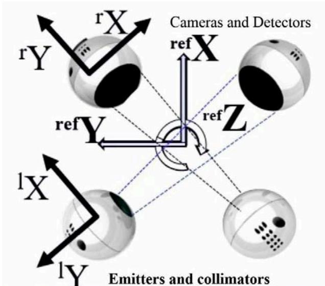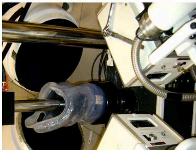Figure 3: Top: The global reference coordinate system ${}^{\mathrm{ref}}\mathbf{XYZ}$ for the biplane system and two local coordinate systems (right single plane ${}^{\mathrm{r}}\mathbf{XYZ}$ and left single plane ${}^{\mathrm{l}}\mathbf{XYZ}$ ) for normalizing the kinematics information; Bottom: close-up view of the actual leading "scanning head" of robotic system with two emitters and two intensifiers positioned by the robots to scan a composite structure; # 2.2 Imaging Protocols-Variable Source to Object Distances (SOD) and Object to Imager Distances (OID) 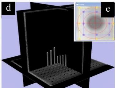The system adapts to meet the requirements of the scanning object, eliminating the need for extensive sample preparation. Programmable adaptable collimators control the exposure and manipulate the field of view (FoV) leading to an overall controlled and optimized emission, suitable for each application based on specially performed calibrations (fig. 4). Figure 4a illustrates the overall setup of the robotic radiographic system, including the X-ray emitter, detector, and a third robot dedicated to positioning calibration grids and phantoms. 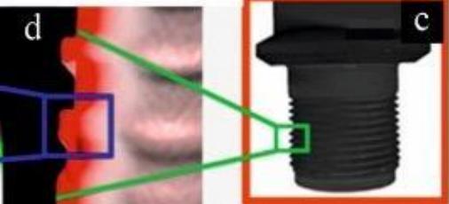Figure 4b shows the multi-marker 3D calibration cubic phantom that contains a 1,145-marker 3D micromachined grid made of polyvinyl chloride (PVC) with accurately (and orthonormally) embedded tantalum markers having diameters ranging from 0.02 to $2\mathrm{mm}$. This cubic phantom is used to determine the imaging geometry of the robotic radiographic system. This cube is also used to correct distortion introduced by the image intensifiers and associated optics [33], [34]. Figure 4c shows the head of one of the rods carrying two calibration markers; the micro-CT image in the background demonstrates the scanner's $10~\mu \mathrm{m}$ resolution capabilities. In Figure 4d, each tantalum marker's position is calculated to determine the system's setup for 3D volumetric reconstructions, while Figure 4e provides a close-up view of a single-plane projection highlighting a tantalum marker's X-ray signature. The system employs geometric and optical magnification techniques with fixed, clearly defined coordinate systems to enhance imaging resolution (fig. 3).    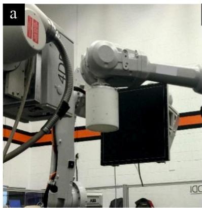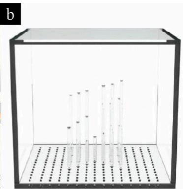Figure 4: Overall controlled and optimized emission/detection approach using multiple robots and specialized phantoms: (a,b) System overview with programmable collimators; (c) Head of a rod carrying two calibration markers-beads, shown with a micro-CT background (10 $\mu$m resolution); (d) 3D reconstruction of the calibration cube with embedded tantalum markers; (e) Single-plane projection revealing the X-ray signature of a tantalum marker.  # 2.3 Emitters and Detectors A selection of different emitters is available, ranging from low power systems to powerful X-ray generation grids for deep layer imaging. For reference we cite here the X-Ray generators that were mostly used in the present work but many more are part of the device options [35]: Max. Voltage 1-160kV with Max Power 300-1.2kW, Max mA 600. Note that a wide variety of focal spots are implemented (ranging for 0.063 to 7.5 mm and micro level applications with the microfocus focal spot sizes reaching $16\mu \mathrm{m}$ ). In the high-energy X-ray CT production option up to 9 MeV, a fine energy bin width of less than $100\mathrm{keV}$ is required with an optimized signal-to-noise ratio (SNR) when inspecting with appropriately tuned focal spot, large and dense parts in deep structures such as those associated with aerospace or automotive inspection work. Detectors include amorphous silicon (a-Si), indium gallium zinc oxide (IGZO), and CMOS sensor type panels, among others. Binning and automatic stitching of images enhance appropriately the resolution and field of view (fig. 3). For reference we cite here detectors that were mostly used in the present work but many more were employed [38]: a) $16 \times 16$ to $43 \times 43 \mathrm{~cm}$ , Pixel matrix $1536 \times 1536$ to $4288 \times 4288$ , pixel size 45 to $200 \mu \mathrm{m}$ resolution, Max frame rate 40 to 160 fps, 2x2 binning 280fps, PAN option 600 fps, active area; b) DC-TDI Photon counting, $102 / 78 \mathrm{~mm} - 1030 / 412 \mathrm{~mm} \times 6$ , Pixel size $100 \mu \mathrm{m}$ , Max frame rate 333-6000 fps, both single and dual Energy; [35] Halide perovskites [39] were also employed due to their strong X-ray absorption and excellent optoelectronic properties (high spatial resolution of $12 \mathrm{lp} \mathrm{mm}^{-1}$ and excellent X-ray imaging properties under a remarkably low X-ray dose of $\sim 50 \mu \mathrm{Gy}$ air, which is just half of the X-ray dose typically used in the traditional flat panel equipment. Coupled with the image intensifiers configuration are specially customized (CMOS) back side illuminated (BSI) camera sensors with $9.27 \mu \mathrm{m}$ pixel size, $2560 \times 1664$ resolution and capacity for $9,350 \mathrm{~fps}$ data acquisition rate. A global electronic shutter with an extreme dynamic range (EDR) make these unique for dynamic imaging. # 2.4 Motion Compensation Techniques Resolving image artifacts (blurriness), motion detection and compensation has been always a huge challenge for both 2D and 3D imaging protocols, from the early days to the most recent stereovideoradiography research [40], [41], [42], [43], [44], [45], [46]. External fiducial markers attached on the surface of the object to be scanned were used in many stereovideoradiography approaches [30], [37], [47] to correct these motion artifacts. The present system employs motion compensation techniques to acquire high-quality images while the object is in motion, i.e., while the object is performing a high-speed load bearing task and is undergoing deformation. This is achieved here, through the accurate (robot's accuracy is $10\mu \mathrm{m}$ positional-geometrical X-ray source-detector trajectory recording during the scan procedure [28], [29], [30], [34], [36], [37]. The relationships between all X-ray components, therefore, are also known with high precision (0.005mm is the robot's precision), allowing for an almost error-free fusion of all imaging modalities. Note that the accuracy and repeatability of the robots reported here is relevant to high speeds of operation at the manufacturing environment. Contrary to these speeds the operational envelope of speed for the robots used here never exceeds $10\%$ of their maximum capacity. This was expected to improve their stabilization and repeatability parameters. The open gantry mechanical architecture of the system allows $360^{\circ}$ visibility so that the high-speed vision system produces highly accurate relationships between the moving object and the detector/emitter combinations i.e., the robotic arms. Practically, what this means is that unlimited trajectories in space between the emitter and the detector are feasible for the first time in tomography. Once the motion is known, the motion compensation is applied at the back-projection step. To minimize motion blur during rapid target movement, the system is also capable of synchronously acquiring 10000 fps from two cameras fixed at the two different robotic arms during movement of the object scanned. This configuration provides a large, open area suitable for either rail-assisted scanning of large sized objects by following them for part of their trajectory or scanning of free moving objects that cross the field of view. The marker-based and markerless motion tracking techniques have been documented elsewhere, [23], [28], [29], [30], [31], [32], [33], [34], [36], [37], [47], [48], [49], [50], [51], but detailed TIC-related calibration and accuracy analyses for both techniques are given here. Experience with this system during these past different-size composite parts studies has shown that adequate data can usually be obtained with a minimum of 1 min X-ray duration, generating estimated entrance exposure of approximately 880 mR/test (times two for the stereotactic biplane mode of the device) for a typical aircraft engine part (turbine blade) study. Such study usually consists of three trials each of two different movement activities resulting in a total entrance exposure of approximately 4-5 R and up to 10 times that magnitude if the blade is scanned through its entire cover, without disassembling. The system, however, can run for more than an hour to scan deep structures and allow for high-resolution, high-density data, depending on the composite structure and depth of the part in question. Although the radiation exposure can be monitored, it was not the case in the present study. A series of studies in the past have enabled for multiple assessments to minimize the total number of trials and Xray generation required for a specific target (type of material, size/dimensions of parts, composite structure, and distribution of material). This comprehensive imaging approach allows for accurate calibration and assessment of different target sizes and materials, while the system's flexibility supports varying scan durations and exposures based on the complexity of each component. The device's KINEDOSE manual, provides the user with numerous protocols (see sample image in fig. 8b) specifying parameters (FoV, dose, exposure etc.) multi-trial testing for several materials [35].    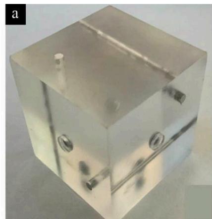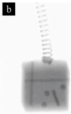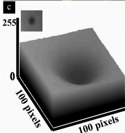Figure 5: (a) Phantom cube showing embedded markers and rods; (b) Radiographic view of the cube; (c) Tantalum marker 3D surface plot illustrating intensity distribution; (d) 3D model overlay emphasizing internal geometry.  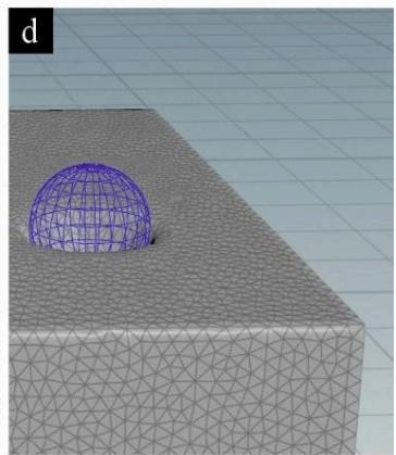In addition, biplane radiographic high-resolution image sequences of a fixator from an aircraft wing component and from a phantom calibration cube of known geometry (fig. 5) were collected using the 3D CT modality to be used for calibration, development and testing. The calibration object (fig. 5a) is a Plexiglas cube with $30\mathrm{mm}$ side and $0.6\mathrm{mm}$ diameter tantalum spheres placed flush in the middle of the top surface of the three orthonormal cubic sides. In addition, tantalum cylindrical rods (0.3mm in diameter) placed flush and parallel to the surface of the three orthonormal sides at 8x8mm from the corners were used for geometric reference; Figure 5b illustrates a biplane radiographic image sequence of this phantom cube of known geometry, acquired via the 3D CT modality for calibration and testing of marker-based and markerless tracking. Fig. 5b highlights how the cube's internal features appear under X-ray during high-speed movement while the cube is suspended from a spring; Fig. 5c provides a 3D surface plot derived from the scan, from a detector with $2304 \times 2304$ pixels resolution, demonstrating the gray level intensity distribution of a selected region with a tantalum marker. Fig. 5d shows a 3D surface model overlay, here visualized with a spherical mesh, to further emphasize the shape and positioning of key internal elements. The ANSA BETA CAE systems software [52] reconstruction of the volumetric cube using tetrahedra can clearly depict the tantalum marker structure and can perform different type of volume and geometry measurements. These one-to-one voxel-to-element correlations are used by the meta-analysis to differentiate between composite layers. The distances between the tetrahedra centroids are also used to quantify geometrically the 3D micro level damages in the structure of the object in question (dimensionality) [33], [51]. The front part of the component and the cube had at least four radiopaque markers (1.6-mm tantalum markers-beads) glued to different areas (internal and external). This allows determination of six DOF motion parameters with high accuracy (errors of 0.01 mm for translation and 0.12 for rotation) using the previously developed marker-based method [27]. A comparison was performed between the marker-based method and the 3D model-based markerless method for evaluation of accuracy on predefined known motion of the cube test. Initially, a CT scan of the target fixator within the aircraft wing structure and the phantom cube were obtained to generate their volumetric model. One thousand and four hundred 0.001-mm-thick transverse-plane slices (2560x1664 pixels resolution, capacity for 9,350 fps, and in different binning resolution could reach 4096x2304 at 1000fps) were acquired from the surface of the part and up to 55 cm below the wing part surface. Segmentation of the CT-scanned target was performed by thresholding the slices to isolate the aircraft fixator from remaining structures. Radiopaque tantalum marker signatures were identified automatically by the software and an operator confirmed their selection (fig. 5, 7, 9). The software replaced voxel values with the mean values from surrounding voxels to eliminate influences of the markers (masking). The volumetric model was resampled using a bilinear interpolation function to the same resolution as radiographic images acquired with the biplane robotics system. The same process was repeated for the phantom cube. The markerless motion tracking technique, i.e., the 3D model-based method assumes that a properly oriented projection through a 3D volumetric model will produce an image similar to the radiographic images. First, imaging geometry of the biplane radiograph system was determined based on a reference coordinate system (fig. 3) [43], [53]. The biplane system was simulated as two single-plane radiograph systems based on these parameters. An overview of the tracking process for the single-plane radiograph system is provided in fig. 6. The algorithm consists of four major components: volume visualization (model projection), image preprocessing, similarity measurement, and optimization. In the volume visualization step, a 3D texture-mapping technique is used to project through the 3D target part volumetric model and generate a digitally reconstructed radiograph (DRR) (adopted from [44], [45]). During the preprocessing step, a set of image processing algorithms (edge extraction, image enhancement) is applied to extract the coarse edge of the target if necessary (fig. 7). In other words, the 3D CT volumetric model collected with the CT modality of the robotic scanner is translated and rotated by 6 motion parameters (3 translations and 3 rotations) using an initial guess and projected to 2D image by the volume visualization method. The produced projected DRR requires some pre-processing (fig. 7) to be roughly segmented the component to be tracked from other parts. Fig. 7a presents (a single X-ray image (out of thousands) from the dynamic stereovideo-radiography sequence showing internal structure undergoing strain; Fig 7b shows a Gaussian filter to identify the major object markers or landmarks to be assessed whereas fig. 7c is identifying the relative object localized strain by assessing the elongation/deformation $(\Delta l)$ of the various object markers or object landmarks forming a mesh at different time instants; Figures 7d-7e illustrate a similar estimation of relative engineering shear strain by assessing the 3D skewness (departure from orthonormality in (e) or initial geometry in (d) of the object mesh; Fig. 7f illustrates how image processing of the grey signature of a cross-like structure at the object mesh in terms of grey level distribution, assists in identifying shear by comparing the mesh at rest (unloaded object, top) and the skewed mesh (loaded object, bottom) [33]; Fig. 7g indicates how the CT model projection is performed. The CT model is resampled with equally spaced planes along the viewing direction and a DRR is generated by summing pixel values along projected rays from the X-ray source to the image plane. Similarity between the DRR and the radiographic image is determined with a correlation. An optimization algorithm iterates motion parameters until the maximum similarity is obtained. Once six DOF of the center point of the target model are estimated from each single-plane system, the absolute 3D position and orientation of the target part in the reference coordinate system are determined using a 3D line intersection method (fig. 10) and the known imaging geometry of the robotic system. Note that the correlation process between two images continues until this iterative optimization finds the optimal similarity.  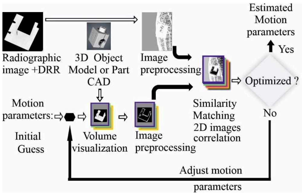Figure 6: Overview of the process for measuring the object position and orientation from the single-plane radiograph system.  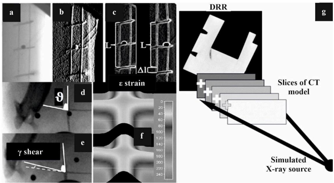Figure 7: (a) A single X-ray image (one of thousands) from the dynamic stereovideoradiography sequence, showing the internal structure of a target under strain or shear; (b to f) show different image processing techniques to detect major markers or landmarks on the target so the resulting relative localized strain and shear can be calculated; (g) CT model projection, where the CT data is resampled into equally spaced planes along the viewing direction, generating a digitally reconstructed radiograph (DRR) by summing pixel values along projected rays from the X-ray source to the image plane. # 2.5 Determination of Imaging Geometry Imaging geometry was determined using the multi-marker 3D calibration cube presented earlier (fig. 5). The calibration cube was put in the view area of the biplane system, and biplane radiographs were acquired. Positions of each marker were calculated to determine the configuration of the robotic system relative to the global reference coordinate system using the direct linear transformation (DLT) method [43]. Each single-plane system, right and left (denoted by "r" and "l," respectively), of the robotic system was described with its extrinsic and intrinsic parameters. Extrinsic parameters consist of the position and rotation of the X-ray source of the single-plane system in the global reference coordinate system. For the right_(left) system, a position vector, $\mathrm{refP_{rs}}$ ( $\mathrm{refP_{ls}}$ ), a rotation matrix, $\mathrm{refR}$ ( $\mathrm{refR}^{\mathrm{l}}$ ), were determined from the DLT method. Intrinsic parameters include the principal point and the principal distance of the single-plane system (fig. 8a).  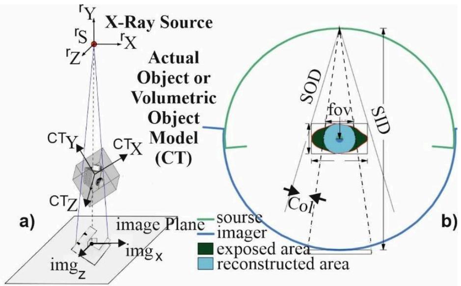Figure 8: (a) Imaging geometry of the single-plane radiograph system (one of the two subsystems in the stereotactic configuration) (b) Geometric magnification by adjusting the SOD and OID. Principal distance (rPD), is from the X-ray source (rS) to the principal point (rPP) in the image plane and the principal point is the origin of the image plane. X axis and Z axis of the image plane are parallel to those of the X-ray source; Notice the projection of the 3D object at the image plane is expressed in an appropriate coordinate system. Geometric magnification is achieved by adjusting the SOD and OID (fig. 8b), while optical magnification uses specialty lenses to achieve different levels of magnification before the signal is recorded at the detector side imaging Protocol example 1: $\mathrm{SOD} = \mathrm{OID}$ , concentric circular trajectories of source and detector about the object (for Cone and Fan-beam configurations). In blue and green solid line, the detector's and source's pathway are depicted respectively. The magnification factor is double and the FOV restricted; when $\mathrm{SOD > OID}$ , the concentric circular trajectories have different radii resulting in significant controlled magnification reduction $(1 < \mathrm{M} < 2)$ and increased FOV with larger volume captured and reconstructed; Collimators (Col) are used to limit beam size to the specific area of the object. The principal point, ${}^{\mathrm{r}}\mathrm{PP}({}^{\mathrm{l}}\mathrm{PP})$ , is the location in the image plane of the right_(left) system, perpendicular to the center of the X-ray beam. The principal distance, ${}^{\mathrm{r}}\mathrm{PD}({}^{\mathrm{x}}\mathrm{PD})$ is the distance from the X-ray source to the principal point of the right_(left) system. The intrinsic parameters, along with the size and resolution of the radiographic image, were sufficient to accurately simulate two single-plane radiograph systems. The extrinsic parameters were used to reconstruct the biplane system for determining the absolute 3D pose of the target in the global reference coordinate system of the robots. # 2.6 Volume Visualization With the geometry of the imaging system known, DRRs can be generated from the 3D target model using volume visualization methods [22], [23], [35], [43], [45], [46], [48], [54], [55], [56]. Perspective (rather than parallel, fig. 7g) projection rendering is required to accurately represent the cone-beam X-ray image formation process. Additive reprojection [54] or ray-casting methods [44], [48] are commonly used for this purpose. However, these methods are computationally intensive, particularly for iterative methods. Restriction of the CT target model to specific regions [22], [24] and/or precomputing a library of ray integral values have been proposed to accelerate the rendering process [23]. However, for tracking arbitrary orientations of large composite parts moving through significant volumes, the computational cost of precomputing the required number of rays approaches that of ray-casting. To significantly reduce rendering time, perspective projections were generated using a hardware-accelerated 3D texture-mapped volume rendering method, implemented using the OpenGL graphics library [35]. The entire 3D model volume data was downloaded into texture memory once. To simulate a desired 3D orientation, the volume was rotated to orient the target properly and re-sampled in memory to create equally spaced planes perpendicular to the principal axis of the X-ray beam. Each pixel of the DRR was calculated by summing re-sliced pixels along a ray constructed from the X-ray source to the image plane (fig. 7g). This reduces rendering time by a factor of about 60, at the cost of a slight reduction in the quality of the resulting DRR (relative to traditional ray-casting). # 2.7 Image Preprocessing The data acquisition rate varies from 1 to 10,000 frames per second (fps), with angular speeds of the robotic arms ranging from 1 to 20 degrees per second. The system processes 450 to 12,000 2D projections in real-time, depending on the application and mode, providing 3D reconstructions within seconds. Using the pulsing X-Ray capabilities, the accumulative exposure time can be less than a second (<1s) and up to several minutes in prolonged scans [32], [33], [38], [53]. The highest accuracy is obtained with the highest repeatability option of the robots tuned to $0.005\mathrm{mm}$ for translation of the robotic arms at less than 1 degree per second rotational speed. Relative to conventional fluoroscopic images commonly used for 2-D/3D image registration [22], [24], radiographic images obtained from high-speed video cameras are less noisy, but still the feature-extraction process can be complicated. This situation can be worsened by the inherent inhomogeneity and anisotropic nature of composite materials. Thus, it is desirable to extract a feature set using all available information on the target composite structure, rather than only external edges or intensity information. This was accomplished by using a combination of edge and intensity information (texture information projected through 3D volume of target model see fig. 7) based on the assumption that even "imperfect" (i.e., highly or less irregular) edge data can serve as useful features for improving matching between the DRR and actual radiographic images. Changing the robotic pathways during image acquisition alters the projection shapes which helps this matching step when dealing with composites. Both the DRR and the radiographic images are preprocessed prior to matching, to maximize similarity. First, the DRR is inverted and contrast-enhanced using a histogram-equalization algorithm [55], [56] (see fig. 6). Then a simple edge algorithm (Sobel edge detector) [55], [56] applied to extract edges from both DRR and radiographic images. The edge information is then added back to the original images (see fig. 7), combining both edge and texture information. The edge information helps to drive the optimization toward the correct solution, improving initial algorithm convergence [57]. The addition of the intensity/texture information leads to more accurate matching than is possible with edge information alone. # 2.8 Similarity Measurement for the marker-less tracking algorithm To determine optimal position matching, a metric for similarity between two images is required. Pattern intensity [24], [58] and gradient difference methods [59] have been suggested for the DRR and fluoroscopic images. These studies assumed that image quality is high, and that composite structures have a relatively small role in the intensity distribution in fluoroscopic images. Because high-speed radiographs can be noisy and at areas contrast-limited, and there is a great deal of composite deformation during dynamic studies, detectable edges and features in the actual radiographs differ from those in the DRRs. Thus, these assumptions are no longer valid, and a different approach was required. Evaluation of several different correlation strategies suggested that general normalized correlation [55], [56], applied to summed edge/intensity images, is robust even in the presence of these differences between actual radiographs and DRRs. The correlation equation used for this study is $$ V(x, y) = \sum_{x,y} \left[ r(x, y) - \overline{{r_{u,v}}} \right] \left[ m(x - u, y - v) - \overline{{m}}\right] \left[\sum_{x,y} \left[ r(x, y) - \overline{{r_{u,v}}} \right] ^{2} \sum_{x,y} [ m(x - u, y - v) - \overline{{m}} \right] ^{2} \right]^{\frac {1}{2}} \tag{1} $$ $\mathrm{r(x,y)}$ radiographic image; $\mathrm{m(x,y)}$ DRR generated from the 3D CT model; $m$ mean of the DRR; $\mathbf{r}_{\mathrm{u,v}}$ mean of radiographic image in the region under the DRR. However, this is computationally intensive, especially if the size of images to be compared is large (as is often the case with images of large composite materials). A new Quadtree-based normalized correlation method was employed to reduce search iterations and improve optimization efficiency. A predefined search space of the radiographic image is divided into four quadrants (fig. 9). Note how resolution affects the size of the acquired tantalum marker X-ray signature. Steps one to six of the process of isolating the high-resolution marker (shown in subgraphs 1-6): 1-2-3: Masking of the marker signature, 4-6: The 5x5 Laplacian filter applied on a small area around the marker's region to enhance the contrast and remove the useless information (background noise) close to the marker. Quadtree-based correlation is also shown. Correlation space is divided into four regions. The region with the best match is subdivided again. This process is repeated until the region size is reduced from thousands to $4 \times 4$ pixels.   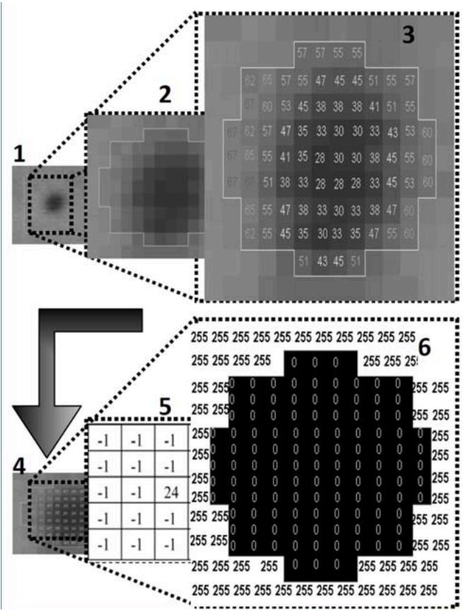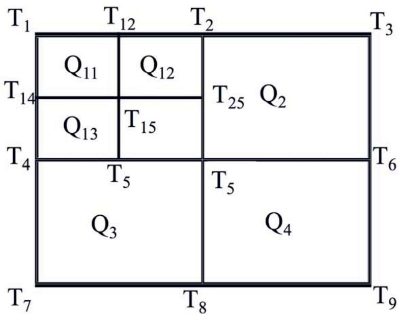Figure 9: Top: Tantalum marker X-ray signature surface plots at $576 \times 576$ and $2304 \times 2304$ pixels, with subgraphs 1-6 showing the masking and Laplacian filtering steps. Bottom: The quadtree-based correlation, where the search space is repeatedly subdivided until a $4 \times 4$ pixel region remains. The average correlation value $(\mathrm{AT}_{\mathrm{q1}}, \mathrm{AT}_{\mathrm{q2}}, \mathrm{AT}_{\mathrm{q3}}, \mathrm{AT}_{\mathrm{q4}})$ of each quadrant (Q1, Q2, Q3, Q4) is calculated from correlation values of four corner points of the corresponding quadrant (equation 2). The quadrant with the best correlation is further divided for the next step (equation 3). For example, if $\mathrm{AT}_{\mathrm{q1}}$ is the optimal, $\mathrm{AT}_{\mathrm{q11}}, \mathrm{AT}_{\mathrm{q12}}, \mathrm{AT}_{\mathrm{q13}}$ , and $\mathrm{AT}_{\mathrm{q14}}$ are calculated. This procedure continues until the size of a quadrant reduces to $4 \times 4$ pixels. In the final step, all pixels of the optimal quadrant of the radiographic image are correlated with the DRR. The coordinate of the pixel with the best match is chosen as the location of the target center in the image plane ( $\mathrm{refP_{rm}}$ and $\mathrm{refP_{lm}}$ see fig. 10).  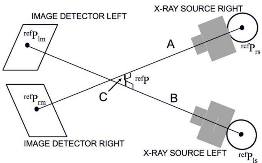Figure 10: Determination of 3D target part position. refPrs(refPls) is the position of the X-ray source of the right_(left) system relative to the reference coordinate system. refPrm(refPlm) is the best-matching location in the right_(left) image plane expressed in the reference coordinate system. The mid-point of the line segment "C" is chosen as the optimal 3D position. The value of the correlation function at this point is used as an indicator of the quality of match for the optimization process described below. For a maximum expected frame-to-frame translation of 200 pixels (400x400 pixel search region), the efficiency of the Quadtree algorithm is clearly illustrated. Conventional sequential correlation would require 16000 image multiplications to find the best matching position, whereas the Quadtree-based correlation method requires only 400 multiplications. This is a significant detail when thousands of frames need to be tracked. At the first iteration: $$ ATq1 = \frac {T1 + T2 + T4 + T5}{4} for quadrant Q1 $$ $$ ATq2 = \frac {T2 + T3 + T5 + T6}{4} for quadrant Q2 $$ $$ ATq3 = \frac {T4 + T5 + T7 + T8}{4} for quadrant Q3 $$ $$ ATq4 = \frac {T5 + T6 + T8 + T9}{4} for quadrant Q4 \tag{2} $$ At the second iteration $$ \begin{array}{l} ATq11 = \frac {T1 + T12 + T14 + T15}{4} for quadrant Q11 \\ATq12 = \frac {T12 + T2 + T15 + T25}{4} for quadrant Q12 \\ATq13 = \frac {T14 + T15 + T4 + T45}{4} for quadrant Q13 \\ATq14 = \frac {T15 + T25 + T45 + T5}{4} for quadrant Q14 \tag{3} \\\end{array} $$ # 2.9 Optimization The downhill Simplex method [57], [60] is used to adjust estimated target part position and orientation until optimal similarity is obtained. The Simplex method requires $N + 1$ points as starting points, where $N$ is the number of DOFs of the function being optimized. Then the simplex method travels through the parameter space by reflection and contraction. Estimating 3D kinematics would typically require simultaneous optimization of all six motion parameters (three positions and three rotations). The optimization routine began with six predefined vertices (as required for Simplex) as the starting points. An initial guess was determined manually for the first frame or selected as the optimal position of the previous motion frame. The remaining five vertices were selected to span the range of valid target orientations. DRRs for each vertex were generated from the 3D model using the known imaging geometry of a single-plane system and five DOF parameters controlled by the optimization process. Then two in-plane position parameters were determined from correlation between the DRRs and the radiographic images. Each reflection or contraction continued to update the three rotation parameters and the distance perpendicular to the image plane, based on the previous similarity calculations. The optimization routine was terminated when the distance of points moved in that step was fractionally smaller in magnitude than some tolerance. To check for local minima, the Simplex routine then restarted from the optimized point and was allowed to converge again. If the new solution differed from the previous solution by more than a specified tolerance (typically, 1 for rotation), the original solution was rejected as a local (nonglobal) minimum, and the routine was restarted from the new optimum point. # 2.10 Three-Dimensional Determination of Position and Orientation Six motion parameters can be estimated from a single-plane system for each frame. However, the assessment of out-of-plane translations is unreliable with a single-plane system and the accuracy for measuring out-of-plane translations is poor relative to the accuracy for measuring in-plane translations [37], [59], [61]. Thus, only a projection ray passing from the X-ray source, through the center of the target model, to the best-matching location in the image plane was constructed from each single-plane system. This projection ray was represented as a line segment connecting the X-ray source (the origin of a single-plane system) and the best-matching location in the image plane $\left({}^{\mathrm{r}}\mathrm{P}_{\mathrm{rm}}\right)$, for the right system and ${}^{\mathrm{l}}\mathrm{P}_{\mathrm{lm}}$ for the left system). For simulating the biplane system, line segments (actually, two end points) estimated from each single-plane system were transformed to the global reference coordinate system based on the information of the position and orientation of single-plane systems relative to the global reference system as follows. - The position of the X-ray source is the origin of the single-plane system. Its location relative to the global reference coordinate system, $\mathrm{refP_{rs}}, \mathrm{refP_{ls}}$ for the right (left) system, was already determined from the DLT method. $\mathrm{^{r}P_{rm}}, \mathrm{^{l}P_{lm}}$ were transformed to the reference coordinate system by a rotation and a translation (equation 4): $$ \begin{array}{l} \text{ref}P_{rm} = \text{ref}R^{r} \mathrm{r}P_{rm} + \text{ref}P_{rs}(\text{for the right system}) \\ \text{ref}P_{lm} = \text{ref}R^{l} lP_{lm} + \text{ref}P_{ls} (\text{for the left system}) \end{array} \tag{4} $$ where $\mathrm{refR}^{\mathrm{r}}$ (refR) is a 3x3 direction cosine matrix expressing the orientation of the right (left) system with respect to the reference coordinate system. $\mathrm{refP_{rm}}, \mathrm{refP_{lm}}$ is the best-matching location in the image plane of the right (left) system transformed to the reference coordinate system. For example, two line segments within the reference coordinate system ("A" from $\mathrm{refP_{rs}}$ to $\mathrm{refP_{rm}}$ and "B" from $\mathrm{refP_{ls}}$ to $\mathrm{refP_{lm}}$) were constructed, as shown in fig. 10. Ideally, the two line segments "A" and "B" should intersect at a point because they pass through the same point of the target model. However, these lines generally do not intersect due to errors such as camera calibration, image noise, matching error, etc. To solve this problem, the 3D position of the target part was determined by finding the midpoint of the shortest line, "C", between these two-line segments using a 3D line intersection method [62], [63] (fig. 10). Orientation of the target part $(\alpha, \beta, \gamma)$ could be determined from the estimated orientation $\mathrm{^{c}tR_b}$ of the target model estimated in each single-plane system assuming body-fixed X-Y-Z rotations [64], [65], [66]. $$ \begin{array}{l} \mathrm{ref}\mathrm{R}_{\mathrm{rb}} = \mathrm{ref}\mathrm{R}^{\mathrm{r}}\mathrm{R} ^{\mathrm{ct}}\mathrm{R}_{\mathrm{b}} \text{for the right system} \tag{5} \\\mathrm{ref}P_{rb} = \mathrm{ref}\mathrm{R}^{l}\mathrm{R} ^{\mathrm{ct}}\mathrm{R}_{\mathrm{b}} \text{for the left system} \end{array} $$ where $\mathrm{^{t}R_b}$ constant $3\times 3$ direction cosine matrix of the orientation of the anatomical target part relative to the CT model; $\mathrm{^{r}R^{ct}}$ 3x3 direction cosine matrix representing the orientation of the CT model with respect to the right (left) system, determined from single-plane optimization; $\mathrm{refR_{rb}}(refR_{lb})$ 3x3 direction cosine matrix of the target part expressed in the reference coordinate system. Final 3D orientation of the target part was determined by averaging the rotation angles obtained from the two single-plane views. $$ \begin{array}{l}\frac{r_m + l_m}{2}\\frac{r_m + l_m}{2}\tag{6}\end{array} $$ $$ \gamma = \frac{\gamma_{rm} + \gamma_{lm}}{2}$$ 2.11 Similarity Measurement for the landmark-based or marker-based tracking algorithm The new MBT algorithm employs image-processing routines (Laplacian filter, Canny edge Detection [27], [44], [45], [55] and homegrown routines to the marker's geometry properties (shape and diameter) (fig. 9). A $5 \times 5$ Laplacian filter was applied on a small area around the marker's region in order to enhance the contrast (fig. 9) and remove the useless information (background) close to the marker (fig. 11).  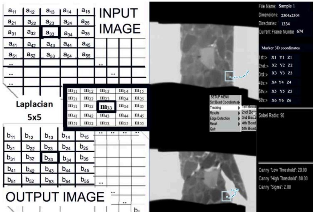Figure 11: The 5x5 Laplacian mask (left) applied on the input image and the output image of the destructive compression granular composite asphalt test (two different views-stereo). The tracking kinematics procedure shows the results from the failed sample shown (right). The snapshot is during the marker tracking and synchronous displacement history of the selected grains from their respective images projected in real time. The plot diagram shown on the right is a collection of points from this tracking. There are approximately 1334 consecutive points during this entire catastrophic event that lie between the points shown here. Figure 9 shows the Laplacian mask applied on an input image and how it manipulates each pixel in order to enhance the contrast. The output image is a result of summarized multiplications among the $5 \times 5$ mask values and the input image (Eq. 7). $$ \text{Output} \left( B_{ij} \right) = \Sigma \left( \text{Input} \; A_{ij} \right) * \text{mask} \left( m_{ij} \right) \tag{7} $$ Figure 11 shows the mask applied over the top left portion of the input image. The center of the mask is placed by the operator over the pixel that will be manipulated. For example the pixel m33 of the mask is applied on the a33 pixel of the input image and the b33 will be finally the new value of the pixel given by Equation (8). $$ b_{33} = a_{11} * m_{11} + \dots + a_{33} * m_{33} + a_{gg} * m_{gg} \tag{8} $$ This software also employs distortion correction and gray scale weighted centroid calculations to improve accuracy and provide sub-pixel resolution [27]. Three-dimensional reconstruction of the 2D biplane displacement history of the tantalum markers is performed with the help of 3D reconstruction software from Motion Analysis (Motion Analysis Corporation, Santa Rosa, CA USA). The algorithm tracks the sequences of images automatically and is an integrated part of the pre-processing toolkit of the robotic system. Static and Dynamic performance of the biplane robotic radiographic system was assessed using the calibration plexiglas with 30mm side (fig. 5) presented earlier. Static precision (a function of system noise) was assessed with the cube positioned stationary in the center of the field of view. Dynamic errors were also assessed by suspending the objects from a spring and then dropping them (increased rotational motion) while allowing them to move freely throughout the field of view. A range of tests was performed using different combinations of acquisition rates, resolution, exposure i.e. 125-1900 images acquired at 400-5000 fps with exposure (shutter) times ranging from 50 to $3000\mu s$. X-ray system protocols ranged from 90 to $320\mathrm{kVp}$ , 40 to 190 mA, 1-30s with low (1152x1152) and high resolution (4608x4608) tests. In the industrial objects tests 3D coordinates of markers were determined for high-speed compression tests using a materials testing machine. ## III. RESULTS Dynamic tests were performed with a phantom target of known geometry (cube). Four tantalum spheres (0.6-mm diameter, fig. 4e) were accurately implanted in the cube to enable marker-based tracking. The texture and cube shape (with implanted parallel rods) were first used for the markerless tracking system. The cube was initially suspended by a spring and randomly moved in the field of view. Alternatively, it was held with a fixed vice attached to a computer-controlled stepper motor driven positioning system capable of two- and three-axis linear movement and multi-axis rotation (0.00635 mm/step, $0.02^{\circ}$ /step). Three types of specific tests were performed: simple translation, simple rotation, and different combinations of translations and rotations. In the translation experiment, the cube phantom was positioned vertically (with one of its implanted rod long axis perpendicular to the ground) and controlled to move parallel to the ground (in the X-Y plane) in diagonal directions along a 100 mm square (smaller squares of 10x10 mm were sampled also). For the rotation experiment, the target was rotated $\pm 10^{\circ}$ internally/externally about its long Z axis (smaller rotations of $\pm 2^{\circ}$ were sampled also). In an example of combined translation and rotation, the target was moved diagonally in the X-Y plane with simultaneous $\pm 10^{\circ}$ rotation about the flexion/extension Y axis. From each experiment, a sequence of radiographic images (1000-2000) was acquired from the biplane robotic radiograph system. For the first frame of each sequence, the six motion parameters were estimated using a window-based user interface to produce DRR that appeared similar to the actual radiographic image. These parameters were used as an initial guess to start the optimization. The optimization routine took on average about 320 iterations for the initial guess and about 560 iterations for tracking the target from frame to frame. The average time taken by an iteration, is a few milliseconds with the biplane image sequences being tracked using the marker-based method described in methods. Our past human arthrokinematics studies have shown the accuracy of this marker tracking method to be $0.01 \mathrm{~mm}$ [27], [51], but we had never tested it with industrial applications. This marker-based tracking used the same calibration cube and distortion correction images as the 3D model-based method, providing a common global coordinate system for comparison. For three tests, the root mean square (rms) differences between methods in the cube experiment averaged 0.023 mm for translation and 0.06 for rotation. In detail, the root mean square errors for the cube experiment between the 3D Model-based (markerless) and the marker based method were in translation (mm): (XY translation: 0.013 in X-axis, 0.03 in Y-axis, 0.02 in Z-axis), (Z-axis rotation: 0.07 in X-axis, 0.13 in Y-axis, 0.06 in Z-axis), (XY translation and Y-rotation: 0.06 in X-axis, 0.05 in Y-axis, 0.12 in Z-axis); and in Rotation (degrees): (XY translation: 0.02 in X-axis, 0.1 in Y-axis, 0.05 in Z-axis), (Z-axis rotation: 0.05 in X-axis, 0.06 in Y-axis, 0.03 in Z-axis), (XY translation and Y-rotation: 0.02 in X-axis, 0.07 in Y-axis, 0.08 in Z-axis). In the dynamic cube study, the calibration cube was randomly perturbed by a spring, causing marker movement through a $1500~\mathrm{cm}^3$ volume (Fig. 5). During low-resolution imaging, each 0.6 mm marker covered at least $64 \times 64$ pixels, corresponding to a pixel size of approximately 0.086 mm/pixel. In the high-resolution setup, each marker spanned at least $200 \times 200$ pixels, reducing the pixel size to about 0.021 mm/pixel. For both static and dynamic tests, the 3D vector distances between pairs of markers were calculated in each frame. In the static high-resolution experiment, the mean measured distance was $29,992~{\mu\mathrm{m}}$ , while under dynamic conditions, it was $29,988~{\mu\mathrm{m}}$ (the true distance is error (20 Hz cutoff), and residual high-frequency errors compare. The consistency of the mean distance between static and dynamic datasets suggests uniform error behavior, while the larger dynamic errors stem from factors such as motion blur, background gradients, and finite pixel-size effects. 30,000 $\mu$m. Typical standard deviations (SD) from the mean distance were $\pm 0.02$ mm (static) and $\pm 0.04$ mm (dynamic). These results remained consistent across the field of view, although both low- and high-frequency noise components were observed in the raw error plots. Fig. 12 illustrates how unfiltered (total) errors, low-pass filtered 30,000 $\mu$ m). Typical standard deviations (SD) from the mean distance were $\pm 0.02$ mm (static) and $\pm 0.04$ mm (dynamic). These results remained consistent across the field of view, although both low- and high-frequency noise components were observed in the raw error plots. Fig. 12 illustrates how unfiltered (total) errors, low-pass filtered errors (20 Hz cutoff), and residual high-frequency errors compare. The consistency of the mean distance between static and dynamic datasets suggests uniform error behavior, while the larger dynamic errors stem from factors such as motion blur, background gradients, and finite pixel-size effects.    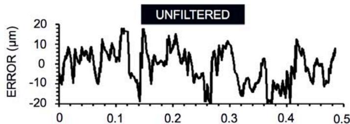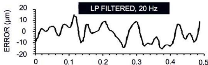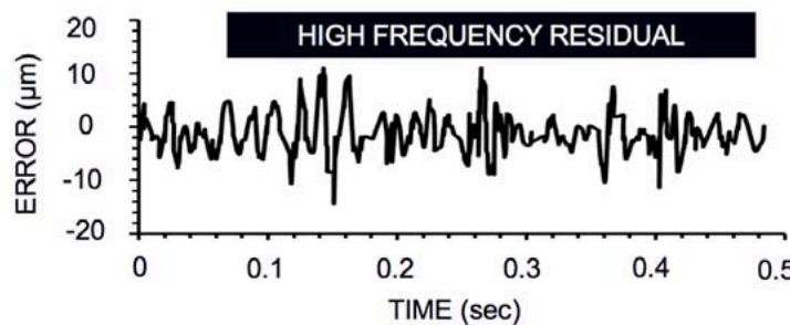Figure 12: 3D errors in the dynamic cube study, shown as the difference between the inter-marker distance for each frame and the mean distance. Top: Unfiltered (total) errors; Middle: Errors after 20 Hz low-pass filtering; Bottom: Residual high-frequency errors. Dynamic errors from all tests averaged $\pm 0.015$ mm (1/40th of the marker size), demonstrating the benefits of gray-scale centroids for finding marker centers with sub-pixel accuracy. 3D calibration and distortion correction were not significant factors, based on the uniformity of the errors across the field of view. Static errors (noise-dependent) were in the order of $0.01\ \mathrm{mm}$ . Dynamic errors were higher than static errors. Motion blur, background effects and quantization errors due to the finite pixel size are the three most likely causes for this. Blur, caused by motion of the markers during the sampling interval, could shift the marker centroid positions. The 2D component of the error is a function of the relative velocity of the two markers parallel to the image plane - if they are moving at the same speed and direction in this plane, both marker centroids would be shifted by the same amount. The 3D distance between two of the test object markers was calculated for every frame in the movement sequence. Low frequency (LF) errors were determined by optimal low pass filtering (approx. $20\mathrm{Hz}$ ) the raw errors. High frequency errors are the residual left after subtracting LF errors from the raw errors. The inter-marker distance would be zero. To estimate the error contribution from blur, the Z (vertical) component of the relative velocities of the two markers was calculated. This axis had the largest velocity component and is also parallel to both camera/intensifier image planes (maximizing the blur effect). The average absolute difference in the Z component of velocity between the markers was $70~\mathrm{mm / s}$ , causing a mean shift in the relative centroid positions of only $0.017\mathrm{mm}$ (at the $500~\mu \mathrm{s}$ sample period). Dynamic error was also estimated for the compression testing described in figures 11, 13, 14. In this case dynamic error was expressed as gray level percentage difference of each marker's centroid gray level from frame to frame; this difference was found to be $2\%$ . Centroid errors can also occur if the materials surrounding the marker are non-uniform in radiodensity. Each radiographic pixel represents the combined density of all objects along the path between the X-ray source and corresponding point on the image intensifier or panel. Thus, the surrounding composite materials will affect the intensity of each marker pixel. A background gradient (due to a curved composite surface or an oblique view of the cube) will shift the calculated centroid away from the true marker center. If the marker crosses a high-contrast object (metals or cube edge), the effect is greater. The low frequency (LF) errors appear to be due to this phenomenon. The frequency and timing of the spikes are similar to those seen in rotational movement plots - for example, the large "dip" in the LF error corresponds almost exactly in time with a sudden $180^{\circ}$ rotation about the Z axis, which then reverts to its previous angle in 0.3 s. Subtracting the LF errors from the total error produces a residual that resembles Gaussian noise. The magnitude of this noise is slightly higher than observed in the static test, due most likely to the finite pixel-size effects that cause small centroid shifts as the marker signature crosses pixel boundaries. The cube study represents the worst-case scenario, with a sharp-edged measurement object undergoing large rotations in all 3 axes and approaching the edges of the calibrated field. Even so, typical errors were in the order of 1/40th of the tantalum marker size. Errors appear to be dominated by the effects of changes in the radiographic background surrounding the marker. Thus, correction for background nonuniformity would appear to offer significant potential for improving accuracy. The other sources of error (noise and finite pixel size) were significantly improved by reducing the pixel size when we acquired higher-resolution images (fig. 13). The average marker area was apparently always greater in the high-resolution tests (fig. 13).  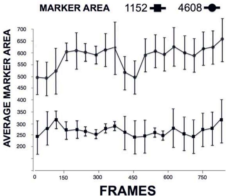Figure 13: Comparison of average marker area between high-resolution (4608x4608-top) and low-resolution (1152x1152-bottom) tests, demonstrating improved centroid accuracy with smaller pixel sizes. Dynamic imaging tests were conducted on various composite materials, ranging from small components to large, multipart assemblies, under destructive (DT) and non-destructive (NDT) conditions involving compression, tensile shocks, and strain experiments. Using the dynamic stereovideoradiography robotic tool, real-time deformation, strain, and shear behaviors were captured. Figures 7, 11, 14, and 15 illustrate these dynamic strain analyses, focusing particularly on the linear velocities and accelerations of individual grains in porous materials during DT and NDT compression (Figure 14). To complement these tests, 3D tomography was performed both before and after loading (Figure 15) to visualize any internal structural changes. In Figure 14, acceleration profiles of various grain structures (positions 1, 2, and 3 in blue, red, and green, respectively) demonstrate how impactful axial loading can produce initial high acceleration peaks (circled regions), which serve as early indicators of potential microcrack formation. A magnified view (middle) highlights these spikes in acceleration, pinpointing the region's most susceptible to crack initiation. In the high-speed robotic dynamic imaging stereovideography destructive setup of fig. 14 a porous cement sample (approximately $70 \times 30 \times 10 \mathrm{~mm}$ ) is placed under compression using an MTS 858 Bionix II testing device. By capturing stereo views of the sample, the system tracks individual grain movements and calculates 3D displacements with an accuracy of about $20 \mu \mathrm{m}$ . This "4D" analysis combines real-time kinematic data with 3D tomography, enabling the measurement of localized strains, shear deformations, and potential microcrack initiation. High acceleration events (up to $500 \mathrm{~cm} / \mathrm{s}^{2}$ ) are recorded, and initial acceleration peaks often signal areas prone to microcracking. Moreover, marker-based and markerless tracking methods can pinpoint the motion of tantalum (or lead) markers or distinct grain landmarks at speeds up to $20 \mathrm{~m} / \mathrm{s}$ , achieving $\pm 0.02 \mathrm{~mm}$ translational and $\pm 0.18^{\circ}$ rotational precision. These capabilities offer insights into how load magnitude, rate, and material composition collectively influence damage progression and structural integrity in composite systems [14], [27], [32], [53].    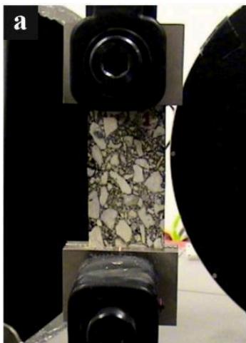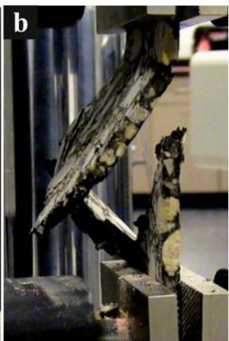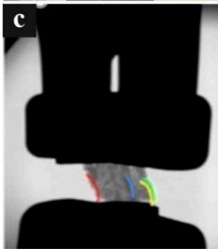Figure 14: (A) High-speed robotic stereovideography imaging setup for DT/NDT compression testing (using an MTS 858 Bionix II device) on a porous cement sample $(7 \times 3 \times 3 \mathrm{~cm})$ . (B) Close-up of the sample's grain structure, illustrating the variety of grain sizes. (C) and (D) Stereo-views of the sample, where individual grains can be tracked and their 3D displacements measured with approximately $20 \mu \mathrm{m}$ accuracy.   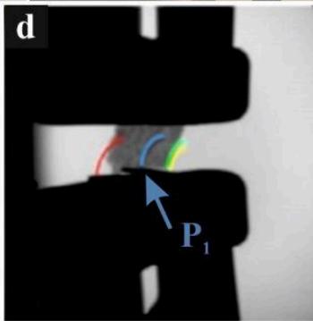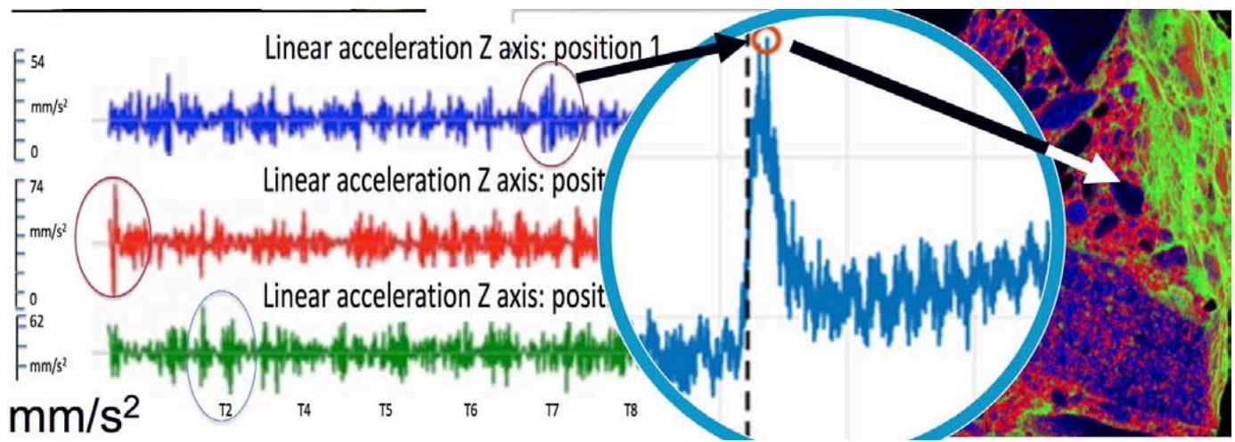Figure 15: Left: Acceleration profiles identifying potential microcrack initiation sites; Right: color-coded map of internal microcrack formation in a composite sample. Fig. 15 compares the acceleration profiles of various grain structures (left) with a color-coded map of microcrack initiation (right) in a composite sample subjected to impactful axial loading. The circled peaks in the acceleration signals highlight high-risk zones where microcracks are more likely to form. By fusing 3D CT data of the sample with the 3D kinematics of these high-acceleration regions, following the method presented in [21], [37], it becomes possible to generate an accurate map of internal microcrack initiation. The grains, represented as colored tetrahedra, correspond to areas of elevated acceleration and serve as indicators of potential microcrack nucleation sites. This integrated approach provides valuable insights into how loading parameters (magnitude, rate), part geometry, and material composition influence the onset and propagation of microcracks. Fig. 16 illustrates a large-structure inspection and part-to-CAD comparison imaging approach applied to the outer exhaust duct of a jet engine—a component composed of synthetic fibers bound by resin. Because this large structure does not fit into conventional scanners, it must typically be disassembled and inspected part by part. The proposed method analyzes fiber anisotropy in high-strain regions, categorizing fibers according to their spatial orientation. In the left part of the figure, a plot shows the distribution of fiber orientations by angle (in degrees), indicating the proportion of fibers aligned at each angle. The middle part employs color-coding to highlight groups of fibers with different orientation angles, revealing areas where anisotropic behavior is most pronounced, and aiding in the detection of porosity, resin voids, or potential delamination. Finally, the right part focuses on the middle layer of fibers, demonstrating a perfectly aligned orientation. This analysis can be used in repetitive stress (fatigue/endurance) tests for these types of materials.  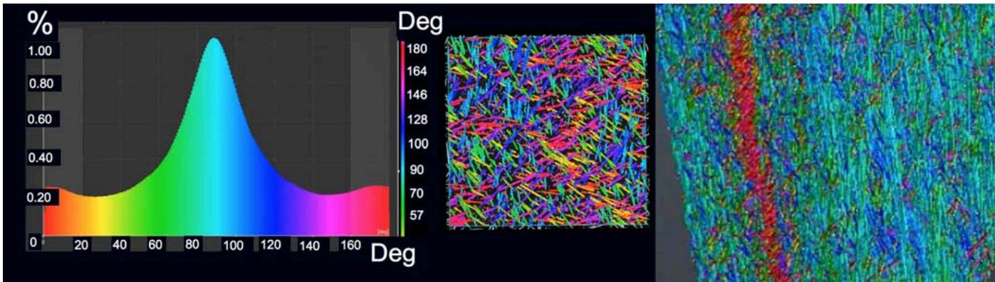Figure 16: Fiber orientation distribution (left), color-coded orientations (middle), and magnified view (right) in a jet engine exhaust duct composite structure. The Part-to-CAD (actual-to-nominal) comparison imaging mode was used to inspect large structures also without disassembling them. This enables the 3D CT scan data of a part to be overlaid with the original CAD model of the same part, allowing for detailed micro-comparisons. Fig. 17 provides a comprehensive illustration of the proposed non-destructive evaluation process. In fig. 17 (a), a single projection captured from a top view can be observed, which clearly shows the distribution of the fixators embedded within the airplane wing structure. Fig. 17 (b) presents a side projection of the same series of fixators, offering additional insight into their spatial arrangement and depth within the structure. The key advantage of this technique is that the 3D tomography scan can be conducted without disassembling the entire structure, meaning that each fixator can be evaluated in situ without the need to remove it for laboratory analysis. This enables to obtain detailed, accurate Geometric Dimensioning and Tolerancing (GD&T) reports that are critical for quality control and assurance. Fig. 17 (c) displays the 3D reconstructed geometry of each fixator, providing a precise model for further analysis. In fig. 17 (d), a close-up view highlights the differences at the edges between the nominal design and the actual manufactured parts, particularly at the threaded areas, with various colors used to indicate discrepancies. Finally, fig. 17 (e) demonstrates a dimensionality analysis where a specific option is exercised to compare the nominal dimensions to the actual measured values along the edges of the fixator. This analysis is carried out with micro-tolerance precision (as fine as $10~\mu \mathrm{m}$ ), and the variability of these differences is presented as a plot along the edge of the material, offering a clear visual representation of the deviation profile.    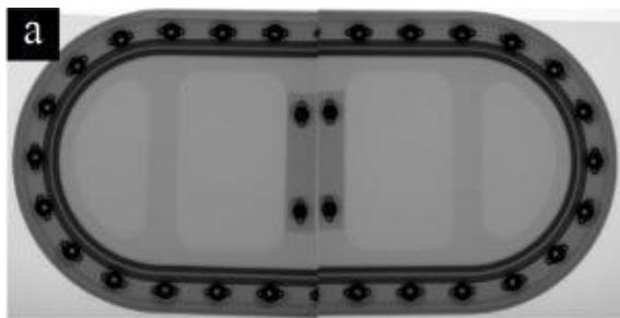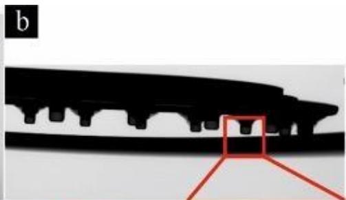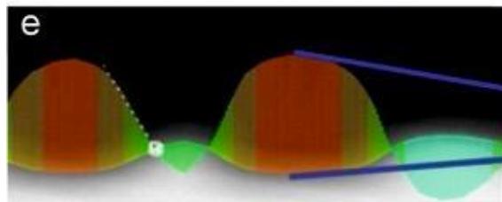Figure 17: (a) Top view and (b) side view projections of a fixator deeply embedded in an airplane wing structure. (c) 3D reconstructed geometry of the fixator; (d) Close-up showing edge differences between nominal and actual parts (thread) with color indications; (e) Dimensionality analysis comparing nominal and actual edge dimensions with micro-tolerance $(10\mu \mathrm{m})$ precision, plotted along the edge.  Data acquisition was completed in approximately 30 seconds for objects within a $2\mathrm{m}^3$ field of view, with 3D reconstructions processed almost in real-time (5-8 seconds including raw data processing and storage). The logged time of previous handling and disassembly labor for that plane part (fig. 17) can take as much as ten days [23]. This initial robotic method for inspection dropped the time to less than half a day including handling and positioning of the robotic scanner around the target. It should be noted that for larger objects, such as a jet engine exhaust duct, inspection durations ranged from 30 minutes to three hours given the need for higher -out of plane resolution i.e., "data density"-, and the need for repeating the tests with alternative trajectories of the emitters/detectors to avoid missing parts of the object. These alternative trajectories were need for calculations for occlusion scenarios and exposure trial and error for optimization of SNR so there was the minimum trade-off and no reduction of spatial resolution. This significant multifold reduction in scan time, comparing to current procedures, is primarily due to the elimination of extensive sample preparation and disassembly. These procedures in conventional imaging techniques can last from several hours, to days or even months, as in the case of Maintenance, Repair, and Overhaul (MRO) A, B, C, D airplane checks [23], depending on the size and complexity of the target. The perovskite detector option presented here has been reported to exhibit the lowest detectable dose rate of $13\mathrm{nGy}$ air $\mathrm{s}^{-1}$ in previous studies, which is over 400-times lower than the medical diagnostic baseline without deterioration in the image quality [39]. Detection efficiency of $88\%$ and noise-equivalent dose of 90 pGy air were also obtained with up to 18 keV X-rays, allowing single-photon-sensitive, low-dose and energy-resolved X-ray imaging. Array detectors like this demonstrate high spatial resolution up to 11 lp $\mathrm{mm}^{-1}$ [60], [67]. Although we did not test these performance characteristics, we note that the detectors were used here in the same configurations and in additional configurations that the radiology dose was tripled or even quadrupled. However, we need to stress that we did not do radiographic dose calibration in the present study. # IV. DISCUSSION CT is finding an increasing acceptance in the TIC landscape, largely due to the evolution of its components associated with resolution, focal point sizes, detector quality, all of which are needed in advanced inspection processes. However certain problems still prohibit its widespread use in inspection related processes, including dynamic accuracy, workflow, gantry size as they translate in the inability to scan large sized assembled targets comprised of composite materials. Robotics-driven multimodal imaging is an alternative to traditional industrial CT scanning that can help resolve some of these challenges. It can combine a series of different imaging modes in one device offering the opportunity to accurately fuse static 3D images (morphology) with deformation and strain data obtained during DT and ND imaging-based testing. This level of automation can help shine light on an actual part, even if it is of large size, resolving internal structures that can be viewed digitally. These internal parts can be visualized and measured with high accuracy, without sectioning or disassembling the actual part from the larger structure that contains it. Inspection of aerospace components, welds in pipes, airplane engines, wings, landing gear and containers can be a demanding imaging task dealing with thick deep layered and/or very dense materials. Typically, hard-to-handle high-energy isotope sources are needed to produce sufficient image quality in reasonable time. Conventional X-ray imagers rely on thicker or specialized high energy scintillators. The trade-off is typically loss of spatial resolution and very laborious time-consuming processes to gather the images. The method presented here offers novel direct conversion technology that preserves spatial resolution even when using a thicker converter layer for improved efficiency in high energy inspection. The necessary geometric trajectory (placement) of this kind of panel detection, however, and its proximity to these highly irregularly shaped structures has been a challenge in the TIC industry. Other challenges include huge scanning times, inability to scan with load bearing and motion, accurate dynamic control of exposure/magnification, and laborious logistics to coordinate disassembly of large components so they can be brought into the laboratory. Even at the laboratory, conventional CT scanners have small-sized gantries for most of these structures. Some structures must also be studied under realistic working conditions. This means impact, vibration or motion at high speeds and load bearing conditions that alter the morphology of the object based on the rate and magnitude of loading, that eventually cause motion artifacts, blurry images, and exposure challenges during imaging. The method presented here can inspect thicker or denser structures with high throughput and a multifold reduction in the scanning time using the photon counting detectors and specialized emitting systems with optimized relationships between focal spot, exposure, detector binning and absorption. The most important solution however, is mainly the ability to control the dosage and compensate for the motion artifacts. Our future studies ought to investigate the interplay of these parameters so that this tool can be fully characterized for a variety of scanning protocols. Automation can help resolve this multiparametric characterization challenge. Robotics-driven imaging can offer combinations of different emitters and detectors in a unique "one-system-many-modalities" imager. The system, therefore, has the potential to unite all these old and new inspection methods in a common reference, both in terms of coordinate systems representing and normalizing the data (fig. 1, 3) and in terms of a hybrid comprehensive inspection platform. The X-Ray data acquisition rate varies, depending on the target and the modality, from 1 to 10000 fps and the angular speed of the robotic system may vary from 1 and up to 30 degrees per second. If we add the robotic arms positioning time that can take from a few minutes and up to an hour (based on target size) the total inspection time can be less than two hours with the actual scan duration ranging from 6 seconds to 30 minutes. In a worst-case scenario that multiple trajectories need to be employed for a complicated composite part like an aircraft structure, the total scanning duration can be half a day including handling and positioning of the robotic scanner around the target. These durations, however, remove from the overall inspection logistics the many hours, and in some cases days, even months required for disassembling of large non-axisymmetric structures so that scanning is possible in conventional small gantry scanners. When imaging occlusion becomes a problem in the presented set-up, a different robotic arm trajectory is selected, and the occluded viewpoint can be bypassed. Fitting a system like this on a mobile robotic imaging station trailer in the future can make this system a mobile TIC facility with flexible open scanning architecture that can approach large structures (planes, pipelines etc.), significantly improving their inspection tasks. A 3D model-based kinematics tracking method was presented in detail as it can help assess the kinematics of a composite target in motion with microlevel accuracy. The method can work for the deep layers of structures as they are visualized with high-speed sequences of biplane radiographs from specialty detectors. The method is based upon optimizing similarity between the radiographic image pairs and digitally reconstructed radiographs (DRRs) generated by projections through a 3D target (generated from CT). However, the matching between DRRs and actual radiographic images can never be exact. The radiographic images result from a combination of the extent of absorption of the different layers of the composite structures, and some level of obstruction of some internal structure on the outmost edges of the target. In contrast, the exact outmost edges of the target can be obtained from the CT volume data, from which certain parts of the composite can be removed. This causes an apparent difference in size between real radiographic images and DRRs (the projected target looked bigger than the target in the radiographic images). This difference varies by frame and is difficult to correct unless we collect radiographic sequences using alternative trajectories which in turn is only possible with an alternative pathway taken by the robotic arms. The high-resolution capacity of the detector has a significant effect on the reduction of these differences and need to be investigated more in a future study. Single-plane implementation of the algorithm resulted in target position estimates farther away from the X-ray source than the absolute position determined using stereo information or marker-based tracking (fig. 10). Thus, assessment of movement perpendicular to the image detector was unreliable with a single-plane system. In figure 10, the target was estimated $2\mathrm{mm}$ farther away from the X-ray source of the left system, causing $0.9\mathrm{mm}$ errors for X axis and $1.9\mathrm{mm}$ errors for Y axis in the reference coordinate system. By combining results from the two views or even more that two trajectories, errors in the beam axis direction are reduced to a level similar to those in the image plane. The two-line segments connecting each projection source and the coordinates of its projections onto the corresponding image plane should theoretically intersect at a point. But these vectors can sometimes not cross, due to small errors from various sources (see fig. 10). During the controlled experiments with the cube described above, these two lines typically missed crossing by only about $0.01 \mathrm{~mm}$ in each axis. Single-plane systems may be somewhat better for estimating target rotation, since 3D rotations calculated separately for each system typically differed by only about $0.03^{\circ}$ (after the estimated orientation from each single-plane system was transformed to the common reference coordinate system). When information from both views was combined, the relative differences between model-based tracking and marker-based tracking data were approximately $0.02\mathrm{mm}$ for the cube experiment for all axes. These errors are similar in magnitude to the effective pixel size of the radiographic images. This suggests that radiographic image resolution may be a limiting factor for accuracy, and higher resolution cameras and/or the addition of subpixel matching techniques can improve performance. It should be noted that this open system architecture enables also dynamic binning options, which in turn allow the same detectors to be used for different imaging modalities with higher resolution results. Binning eventually improves the signal to noise ratio and provides better total image contrast resolution, with the trade-off being reduced spatial resolution. The two magnification modes however (geometrical and optical) can be applied with a tomosynthesis scan of the object in question at the exact same testing set up adding only 30s to 5 minutes of extra imaging time depending on the size of the target. Tomosynthesis provides however, the high-spatial microCT level resolution data that the previous scanning options could not deliver without having to disassemble the part, and/or move it to another scanner in a different laboratory site. More work in the future is required to demonstrate the effects of binning, optical magnification and tomosynthesis in industrial imaging. The blur-motion artifact solution i.e., the capacity to directly measure the 3D morphology of a structure under loading/movement conditions (up to $20\mathrm{m / s}$ speeds) opens a new chapter in the hypotheses underlying the material characterization instrumentation. We believe that much more work is required to reach a golden standard of this methodologies for the plurality of objects and conditions that it can be applied to. An enormous calibration task lies ahead with regards to thickness of specific materials and their composition. Another advantage of controlling the exposure during different stages of the trajectory of the emitter/detector couple is that it offers an indirect way to control the frequency dependence on attenuation. Controlling dynamically the focal spot combined with optical magnification with special lensing systems that in turn have dynamically controlled amplitude, delivers micro-CT capabilities for the first time outside the laboratory and for on-site inspection. More work ought to be performed to demonstrate this capability in detail in a separate study. The spatial resolution (sharpness) alternative is offered where contrast conditions are not ideal. Image "density" (out of plane resolution) can be drastically improved and several times greater than in a conventional system. This is possible because the robotic arms and data acquisition speed can be altered to collect hundreds of thousands of projections if needed. In the metanalysis only the projections need for proper reconstruction are selected, potentially removing the inappropriate motion error projections. The radiographic quantum mottle effects or noise can be tackled by having the grid system, tubes, and collimators of each emitter fire not in synchronicity but with time latencies so the signals from the two different tubes in the stereo system do not cross and do not collide [51]. Its assessment needs also quantification in a dedicated study. A new challenge, however, is associated with the capacity for continuous, autonomous, and excessive use of the detectors and significant need for cooling structures on the tubes. The system literally "burns" very fast through detectors as it is using them at the top of their capacity all the time. That introduces panel disadvantages (as compared to image intensifiers -IIs) that include defective image elements, higher costs and lower spatial resolution if they do not get replaced on time (at least twice annually for a constantly scanning device). The present alternative tool for non-destructive inspection, composition analysis and analysis of carbon fiber parts helps locate the exact axis and point of porosity, resin voids and delamination within complex geometries inside of carbon fiber. Alternatively, it offers reverse engineering and tolerance mapping methods when the CAD model of the part is not known and needs to be approximated from existing geometry. The new robotic imaging system demonstrated an alternative way to study fatigue, impact and any associated deformation, linear expansion or phase change that a material experiences due to the application of different forces at different loading rates using image-based NDT. The time savings of these new methods described here contribute to drastically lower labor requirements and can increase the capacity of a single system, so more parts could be inspected. # V. CONCLUSION In conclusion, the proposed robotic multimodal imaging system presented in this study offers a transformative approach for inspecting large aerospace structures and complex-shaped objects. By integrating advanced motion compensation and dynamic kinematics tracking, the system significantly reduces scan times, improves workflow efficiency, and lowers inspection costs while delivering high-resolution analyses of key material properties such as porosity, dimensionality, and failure modes. The ability to automatically stitch 2D/3D radiographic images into panoramic views of large, non-axisymmetric objects further enhances its utility for reverse engineering and comprehensive quality control. Comparative evaluations between marker-based and markerless motion tracking methods indicate that the markerless approach achieves comparable accuracy, demonstrating its potential for more streamlined and less invasive inspections. These findings have broad implications, with applications extending beyond aerospace to fields like defense, cargo safety, petrochemical logistics, and medical device manufacturing. Future studies will focus on validating the system using a library of standardized target models tailored to specific density and absorption characteristics. This effort aims to establish a simplified, expedited, and cost-efficient standard for dynamic inspection protocols in both laboratory and on-site environments. # ACKNOWLEDGEMENTS This work was supported in part by the US Army Medical Research and Material Command, MOVE Center Award: #07-2-01; US Department of Defense - TATRC Contract W81XWH-07-2-0113, Department of Health and Human Services, National Institutes of Health, EUNICE KENNEDY SHRI-SBIR Award #R44 HD068150-01; Meat and Livestock Australia 2019 Awards #P.PSH.0914 and #P.PSH.0915; the authors would also like to thank Cadence Inc., BETA CAE Systems for their software suite donation and Boeing Inc, for components for tests performed with contributions from SetAero, Shane Arthur at Shimtech/Boeing and KINEMAGINE/ATLAS for providing all the instrumentation and CAD files, in memory of coauthor Fernando Viveros and Prof. George Athanasiadis from BETA CAE Systems.

Generating HTML Viewer...