

IntelliPaper
Abstract
This paper describes an effective approach for model order determination, which allows identifying the dynamical behavior of the mechanical system by using observation input-output data. The concept is based on the minimum means square error of the estimated transfer functions, which can effectively tackle measurement noise and modelling errorsto identify appropriate low-order transfer functions of the structures via an Auto-Regressive Moving Average eXogenous (ARMAX) model. The effectiveness of the proposed method is validated exclusively using experimental data obtained from a grinding test of an industrial manipulator SCOMPI robot. Some other common criteria,such as the Akaike Information Criterion (AIC), the Bayesian Information Criterion (BIC), and the Noise Order Factor (NOF), are investigated in order to verify the performance of the propose methodology. The results show that the proposed technique is cost-effective in terms of optimal model order determination, while the ARMAX model turns out to be the most appropriate representation for feature extraction at the low order. Thanks to its flexibility in handling model disturbance, the proposed optimization strategy is able to capture all the dominant oscillation modes of the structure at themlow orders, and system modal properties are efficiently and automatically determined, while the performance of the ARX model is shown to be less efficient when working at the low orders.
Explore Digital Article Text
I. INTRODUCTION
Operational Transfer Functions (TFs) or Frequency Response Functions (FRFs) of mechanical structures play a vital role in understanding the dynamic characteristics of the systems and in solving general vibration problems during the operational process. They constitute an effective tool aiding the extraction of modal parameters. Estimating the transfer functions of a mechanical system has thus become an important task in many engineering applications. Different representations of transfer functions are crucial in the description and analysis of system properties. In industrial applications, a measurement of the transfer functions defining the structure properties in the frequency domain can be implemented using vibration instrumentations. Different methodologies are proposed in the literature with the aim of estimating operational transfer functions, with the most common applying the Fourier analysis. The Empirical Transfer Function Estimate (ETFE) is a natural nonparametric method that identifies transfer functions by taking the ratios of the Fourier transform of the outputs to those of the inputs [1]. However, this method requires more data points and raw ETFE estimates are generally not accurate enough. With these estimates, the variance does not decrease as the number of data points increases because they contain no information compression feature. Researchers have conducted various experimental studies on structural dynamics under operational conditions. In [2], the FRFs of a flexible joint industrial manipulator with a serial kinematic were identified based on a non-parametric closed loop. However, due to the nonlinearities of the robot, the method faced a challenge in eliminating disturbances in the estimated FRFs. Operational Modal Analysis (OMA) is another approach for identifying the modal properties of the structure using vibration data obtained under operating conditions. Yili Peng et al. [3] identified in-process FRFs based on the OMA and Experimental Modal Analysis (EMA), which uses the natural frequencies and damping ratios to build FRFs under operating conditions. A simulation of a three-degree-of-freedom-mass-spring-damper system and experiments on a machine tool are adopted to verify the proposed method. Similarly, Zaghbani et al. [4] used OMA in the identification of the dynamics of a milling machine under a cutting process work. At the same time, another method was presented in [5] to generate FRFs from identified poles and zeros in the low-frequency domain. Recently, Coppotelli et al. [6] proposed an approach for estimating FRFs from operational data by changing different mass and stiffness distributions. This method also allows evaluating the modal parameters of the structure via operational modal testing. Conversely, Özşahin et al. [7] introduced a new technique to calculate the variation in tool point FRFs under different working conditions by using an inverse analysis of self-excited chatter vibration. In their method, chatter frequencies were experimentally determined and applied to estimate tool point FRFs on 5-axis milling machine via the relation between the measured force inputs and acceleration outputs. However, the tool point FRFs are not well estimated at high spindle speeds due to the presence at those speeds of a low signal-to-noise ratio and the bandwidth limitation of the dynamometer. Another in-process FRF identification approach of the spindle structure was presented in [8]. In that case, the tooltip FRFs were identified under operational conditions based on an inverse solution of critical stability limits. The method is helpful for predicting the stability of the tool holders when the direct measurement of the tool point FRFs is uncompromised. Parametric estimation methods constitute another system identification class. In these methods, it is suggested to use time series modeling for the mathematical description of the transfer functions. It combines the advantage and information obtained from both measurements and theoretical modeling. Depending on the availability of the measurement signals, the Auto Regressive model (AR) [9, 10] or the Auto Regressive Moving Average model (ARMA) [11] can be used if only the output is available. In [12,
13], a modal analysis was conducted in different industrial structures based on three Auto-Regressive Moving Average methods, namely, the recursive least-square, output error, and corrected covariance matrix methods to determine the optimal model order. Conversely, in the case of measurable or identifiable excitation forces, the Auto-Regressive eXogenous (ARX) model [14] can exploit, by assuming that the model's errors and disturbances are white noise. However, because of the unavoidable noise contaminated in the measured signals, the quality of estimated FRFs can be adversely affected by noise originating from the test environment. When the system operates in an industrial condition with a lot of disturbance, identifying the transfer functions of a complex structure may become difficult.
In this paper, we present an original method designed for automatically extracting the modal parameters from identified transfer functions based on the concept of the optimal ARMAX model. Particular attention is paid to selecting optimal model orders, which can closely reflect the dynamic system. The work contributes to the determination of a model order based on the estimated transfer functions, by using the framework of the ARMAX model. The proposed method is experimentally applied to a robot during its grinding operation, and the results are compared to those of the original ARX model. The measured grinding forces may be considered the exogenous inputs excitation, and the disturbances of the system are taken into account by adding the Moving Average part into the model. The estimated orders are verified based on the most common selection criteria, such as the Akaike Information Criteria (AIC) [15], the Bayesian Information Criteria (BIC) [16], and the Noise Order Factor (NOF) [17]. In this study, the ARMAX model is expressed in a convenient way for computation at the low orders, which gives a more parsimonious representation and helps improve the modeling performance, with less computational complexity. We have organised the rest of this paper in the following way. The motivation for the research is established in Section 2 through a detailed description of the time series modeling, with a focus on the ARX and ARMAX models. Section 3 proposes an original method to determine an optimal model order of the mechanical system. Experiments are then conducted on the flexible manipulator, SCOMPI, under grinding operation to validate the proposed methods in Section 4, followed by the identification procedure and the results. We end by drawing several conclusions from this research.
II. TIME SERIES MODELING
System identification is the art of modeling a dynamical system from raw time series data. We consider the problem of estimating a dynamic system model based on the measurement of an N points input-output data, which will be pre-classified into input and output
Various representations of linear time series such as Auto-Regressive (AR), Auto-Regressive Moving Average (ARMA), Auto-Regressive eXogenous (ARX), and Auto-Regressive Moving Average eXogenous (ARMAX) can be employed to extract dynamic parameters . Since there are various time series data types, we should choose an appropriate model. In general, such models are based on an Auto-Regressive (AR) part or output, an eXogenous (X) part or input, or a Moving Average (MA) part or error term, depending on the situation. The AR model is the simplest time series representation, which linearly depends on output data (the vibration responses). In the availability of both input (the measurable and known excitation force) and output data, the ARX model is usable. It is possible to combine these models with the MA term and produce the ARMA representation for the output-only cases and the ARMAX model for the input-output conditions. Once the most appropriate modal structure is selected, we can apply a model to the measurement by minimizing certain criteria:
where is the unknown parameter vector of the parametric model structure.
In automatic control applications, given the current state and input signal, the model can be applied to predict the output of the system by choosing a cost function in the form.
where represents a filter that removes unwanted properties in the measurement data, and is a convex function.
A common representation of the Linear Time-Invariant (LTI) system can be expressed in the from of the linear transfer function model:
where q is the forward shift operator, that is, . Here, is a dimensional vector of output, is a dimensional vector of input, and is the disturbance sequence with an appropriate dimension and assumed to be an independent and identically distributed stochastic process, respectively. Furthermore, the transfer functions and are rational functions in the backward shift operator q, and the coefficients are given by the elements of the parameter vector .
The predictor associated with the output is given by [18]
This model structure is quite general, but we can develop some special cases. A simple case is the ARX model structure, which is:
that can be rewritten in a more general polynomial form as:
where
are autoregressive and exogenous matrix parameters, with I denoting the identity matrix. , , and are the orders of the ARX model, is equal to the number of poles and is the number of zeros, while is the pure time delay in the system. Since and , the predictor of the output can be written as:
where
When the noise is assumed to be a white Gaussian process with zero means, which is uncorrelated with the regressors, the model parameters are estimated via the Least-Square (LS) estimator [19]:
The variance represents the remaining un-modelled behavior of the data.
The corresponding transfer function is . (15-a)
However, in this case, only the deterministic part of equation (1) is estimated by considering no noise . If a noise model is sought, additional steps are needed, assuming that the noise is described by a Moving Average process , which results in an ARMAX structure:
and its polynomial form
where
is the polynomial of order which represents for Moving Average term.
(18) In contrast with the simpler ARX model, this presentation form offers a noisy transfer function , which allows representing different types of noise characteristics through a proper choice of the MA polynomial term. In engineering applications, it is unavoidable when environmental noise contaminated in measured data. Therefore, a parametric system identification algorithm should be adopted to identify the modal parameters from the noisy data. Under this condition, the ARMAX model with real-time identification proves to be efficient. Figure 1 presents the structures of both ARX and ARMAX models.
![Fig. 1: Model structures of ARX (a) and ARMAX (b) [18]](https://doc.journalspress.com/zcao87_67371/ocr/images/derivatives/5c/5ce26056f0a440960a96a68fd2ee4363a6eb10faa3cbb82c8138262e704c3fd7.webp)
If only the ARX model is use, the noise model is described as , where is also used as the denominator of describing the dynamic model. This model implies that the polynomial form must be an average estimate of the poles of and . However, the noise model can be better estimated using the ARMAX model, as described by the numerator polynomial term . When parametric methods use for model estimation, the transfer functions to be estimated are defined as a function of a parameter vector . For the identification of the value , and are closest to , and . In [20], the authors showed that under reasonable conditions,
where and is prediction error and defined in equation (4). According to [21, 22], with this definition of , it is possible to split the total estimation error between the true frequency response function and the estimated one into two parts as follows:
III. A MODEL ORDER DETERMINATION APPROACH
(21) As we can see in equation (21), the errors in the estimated FRF have two components. The first contribution is the bias contribution, a deterministic quantity due to the modeling error. If the selected model has a lower or a higher complexity than the true system, this bias error will be present at some frequencies. Choosing the model order should be flexible enough to allow a good fit to the measurement data but adequately constrained so that noise does not invoke unsuitable models. Consequently, selecting an optimal model order respecting this compromise is an important issue in system identification. This concern is analyzed in the following section to select the optimal model orders of an ARMAX model. The second contribution represents the noise or variance errors, which are due to noise in the measured input and output data. It is a random variable that will disappear if there is no noise or if the number of data tends to infinity.
When time series modeling ARX or ARMAX models employed, the performances may be affected by selecting the model order. Choosing a sufficient and correct model order has always been a challenging issue. Once the model orders are properly selected, the models successfully represent the underlying phenomenon with the lowest complexity. This method aims not only to find a model capable of describing a specific set of data but is also helpful for the validation of the inference procedures. Consequently, there is a need to develop a reliable method to identify the orders of AR, MA, and eXogenous polynomials. In general, most of the mechanical structures are operated in the low-frequency range with limited bandwidth. Having a model with orders that are too high may lead to an overfitting problem as it includes too much irrelevant oscillation information and generates high computational costs, and a model with orders that are too low will not be solid enough to capture the underlying physical system dynamics. For its part, a model with an appropriate order can precisely describe the dynamic characteristics of the system. Because of its important role in system identification, model order determination has attracted much attention in the literature, with researchers proposing different criteria for order determination [23]. The final prediction error (FPE) criterion was originally proposed by Akaike [24] for determining the AR order and was extended to the ARMA model by [25]. After adding the inflating effects of estimated coefficients, the optimal order was chosen by minimizin the one-ste-ahead mean square forecast error. A method based on the eigenvalues of a modified covariance matrix, which is robust to noise levels, was proposed in [12, 13] for determining the model order. Some other concept as information theory like Akaike's Information Criterion (AIC) [15], Bayesian Information Criterion (BIC) [16] or Minimum Description Length (MDL) [26] were developed to produce an estimate model order. Among these techniques, the AIC is a heuristic approach, which has attracted much attention in the literature. His technique penalizes the likelihood of the number of parameters in the model by attempting to choose the most suitable model order.
Considering an N-dimensional time-series data, the AIC is given by equation (22):
where N denotes the number of data points, is a dimension associated with the vector of unknown parameters to be estimated and
is the covariance matrix of the innovation sequence associated with the estimated coefficients, the w[t] is innovation square, or the model error.
When the AIC value is at a minimum, we obtained the most suitable order. A minimum AIC is theoretically situated at a sufficient value of that best represents the dimension of the unknown parameters. For an ARMAX model, would typically be equal to , with and orders for its AR, MA, eXogenous components and time delay, respectively, while p represents the number of orthonormal functions by which each of these components is multiplied. Here, it should be noted that although there would be many possible combinations of and that can produce the same adequate value of , only the right combination would yield the smallest AIC value. The z value may be defined as:
The AIC corresponding to an ARMAX model is written here as:
where z is the number of scalar parameters in the ARMAX model.
However, in many cases, AIC does not give an optimal order. [27] showed empirical evidence that AIC tends to pick models which are over-parameterized. The BIC overcomes this shortcoming by including an additional term that
(25) In this paper, it is written as:
penalizes the model complexity and enhances the procedure, which are based on the same concepts governing the AIC but are better suited for large data sequences. The BIC criterion has the following general form:
These criteria rely on the evolution of the error covariance, which monotonically diminishes concerning the model order. It asymptotically chooses the correct order model if the underlying multiple time series has high dimensions but tends to overestimate the model order as the data length increases. Thus, selected model orders can be greater than the optimal model orders.
However, attention has recently shifted to the equally important problem of bias resulting from
(27) under-modeling. Wahlberg and Ljung [28] have conducted excessive research on the distribution of bias and variance in the estimated transfer function.
In this paper, we present an improved approach to determining time series model orders based on means square errors of the estimated transfer function. This approach is different from traditional criteria such as AIC and BIC. We transformed an averaged frequency means square error on the estimated transfer function into a mean square output prediction error criterion.
The proposed method allows extracting the modal residuals with a sufficient order that guarantees the extraction of uncorrelated residual samples and the avoidance of an overfitting problem. The selection of the optimal order is based on a minimal variance of the total mean square error (1, 2)
\varepsilon\left{\left|\left(q\right)-\left(q,\right)\right|^{2}
\triangleq \int_{-\pi}^{\pi} \hat{\mathbf{E}}{p{o}}(\omega) (\omega) d\omega
The optimal order obtained when:
The aim of this technique is converting the bias error into a random variable by ascribing a prior distribution to it. Consequently, we obtain an estimate for the average characteristics of the total errors. We assume that the transfer function represented by is a stochastic process indexed by the variable , and given some value of , it can be decomposed as the sum of a parameterized plus the residual :
where is a zero-mean stochastic process:
Each system will provide one realization and analogous to the embedding of the single noise realization in a stochastic process. In the framework of an ARMAX model, for ease of implementation, we restrict our consideration to the linear model structures of the Single Input Single Output (SISO) case. The question of computing asymptotic variance expressions in the presence of under-modeling for transfer function prediction errors in frequency domain identification is addressed in this paper. The discrete linear transfer function of the ARMAX model can be expressed in the following form:
The true transfer function can be expressed by the relationship between the measured input and output of the system:
The means square error between the true and estimated transfer function in (28) is calculated by the following equations:
This index is an effective criterion since it includes the stochastic participation in the denominator by adding an input power spectral density .
We converted a average frequency means square error criterion on the estimated transfer functions into a mean square output prediction error criterion. Due to the presence of measurement errors, the proposed method is adopted to determine the optimal model orders and proved its robustness to parameter uncertainties. This modification bridged the connection between classical variable selection criteria such as AIC and BIC and the non-concave penalized likelihood methodology that allows greater flexibility in choosing the desired models. The goodness of its performance will be assessed in the next section through a comparison with traditional validation methods. The optimal model will be tested by the quality of the residuals, the histogram, and autocorrelation functions.
IV. INDUSTRIAL APPLICATION ON A SCOMPI ROBOT
4.1 Description of the test structure
Flexible manipulators are employed in the maintenance of large hydro electronic equipment as they represent an effective solution for repair jobs . Despite their attractive properties, controlling lightweight robot manipulators is still a challenging task. Their flexibility induces structure vibration that deteriorates the trajectory tracking accuracy and may lead to instability issues. In this part, the present method is adopted to identify the dynamic behavior of a light, portable, track-based multi-process manipulator named SCOMPI (Super-COMPact Ireq) . The dynamical transfer functions and modal parameters must be monitored during the grinding process to control vibrations. Figure 2 presents the working envelop and the construction of the robot, with its links and joints.
![Fig. 2: Structure of SCOMPI robot [29-31]](https://doc.journalspress.com/zcao87_67371/ocr/images/derivatives/e4/e46a3891e75419119949160aff0f7881f833ac82d7a28fbd063c32a2bbf459bf.webp)
4.2 Experimental procedure
The tool contact point Frequency Response Functions (FRFs) and their modal parameters represent the key for solving the dynamics analysis. In this paper, the actual grinding forces are used as the input excitations in estimating the FRFs. The grinding test is performed at the 3225 rpm rotating speed with an average 0.08 mm axial depth of grinding cut. The grinding work is realized on a hard steel EN31-64HNC workpiece with the dimensions of 150 x 7 x 48 mm. During the cutting operation, cutting forces are measured with a type CH8408 3-axis Kistler dynamometer, which is directly attached under the workpiece to record the normal force direction ( ), the tangential force direction ( ) and the axial force direction ( ). At the same time, three
PCB-352C34 piezoelectric sensors with a sensitivity of 5.29 mV/G are used to measure accelerations at the robot's end-effector ( ) to capture the vibration in three directions. The measurement is conducted through the LMS data acquisition system for 10 s at a 512 Hz sampling frequency. Figure 3 shows the actual experimental setup of the SCOMPI robot under a real grinding operation. An LMS test lab system was used for acquiring the data in real-time during experiments, as well as for calculating averaged FRFs, which were used to validate the estimated results of the proposed approach.
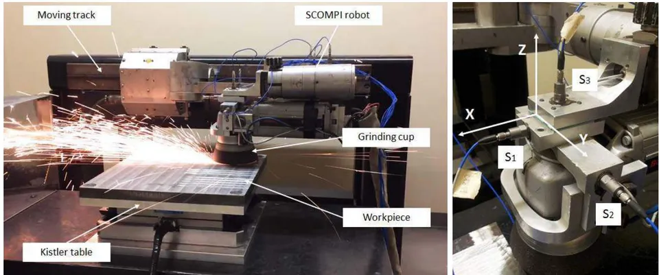
The structure is excited through a grinding operation, during which all the effects related to the rotating tool or the grinding process are considered. FRFs are obtained during the cutting operation through the relations of the cutting forces and the vibration responses. The measured cutting forces are taken as the excitation sources of the system. In this paper, the operational FRFs are determined from the relation between the cutting forces and responses through the time series ARMAX modeling. The detailed experimental description is provided in Table 1.
| No. | Experimental description | Information | Units |
| 1 | Grinding cup (Norton BuleFire) diameter | 12.7 | cm |
| 2 | Workpiece material | AISI 1081 | - |
| 3 | Density of AISI 1081 | 7.87 | |
| 4 | Workpiece dimensions | 20.32 x 25.4 x 2.54 | cm |
| 5 | Grinding direction | Normal direction | - |
| 6 | Power | 500 – 3400 | W |
| 7 | Length of cut | 16.2 – 18.5 | cm |
| 8 | Width of cut | 1 – 1.55 | cm |
| 9 | Depth of cut | 0.0158 – 0.00165 | cm |
| 10 | Rotation speed | 3225 | rpm |
| 11 | Angle of grinding cup | 5-10 | degree |
{"image_source":{"path":"images/1224bcb25343ba3eb33066d8cc1267e3c9d66f1bd6592013998e754100a04a92.jpg"},"content":"","chart_caption":[{"type":"text","content":"(b)"},{"type":"text","content":"(c)"},{"type":"text","content":"Fig. 4: Measured data on SCOMPI robot"}],"chart_footnote":[]}
V. IDENTIFICATION PROCEDURE
5.1 Model orders estimation
The parametric identification of the structural dynamics is based on force and response signals with a 10s sample length. The modeling strategy consists of the successive fitting of the ARMAX model. First, the model orders are selected based on the Akaike Information Criterion (AIC) and the Bayesian Information Criterion (BIC). Figure 5 plots result from the AIC and BIC techniques respectively obtained by directly fitting the ARMAX model of increasing orders p = 1 - 60 to the different sets of experimental data.
{"image_source":{"path":"images/460269222dd2a4edbe38ec29248f569f242563e5184a8abdf3c069223a393eae.jpg"},"content":"","chart_caption":[],"chart_footnote":[]} {"image_source":{"path":"images/0c445fd2d4556a6e934b50888d4379f08b80693950021b0cd705687bc539cc11.jpg"},"content":"","chart_caption":[],"chart_footnote":[]}
{"image_source":{"path":"images/d4cdb76f501e83ea0b2245cb0151e381ed2351c01a9c4ac2feed31a8453a1b11.jpg"},"content":"","chart_caption":[{"type":"text","content":"Fig. 5: Model order selection based on AIC and BIC criteria for different sets of data: (a) X data, (b) Y data, (c) Z data"},{"type":"text","content":"Optimal ARMAX Model Order Identification of Dynamic Systems"}],"chart_footnote":[]} By dividing the experiment into different test directions based on the operation of the robot, we can decompose and characterize the dynamical behavior of the system for each direction. From Figure 5, both the AIC and BIC methods decrease with the model order, and a minimum may be assumed close to 47. However, the main limitation of using such techniques is that they may suggest different model orders and not determine the optimal orders. Thus, these values must be judged carefully.
{"image_source":{"path":"images/3a4f7d042378c867ed1d31c9a620da00d7f4e22da20e5fdfa9b523a4792152c2.jpg"},"content":"","chart_caption":[{"type":"text","content":"(b)"}],"chart_footnote":[]} By applying the proposed method in selecting an optimal model order, the orders for which all curves lead to a stable value are identified. Figure 6 illustrates an optimal order, defined as the smallest order value. The point of convergence starts at around order of 10 in all three directions.
{"image_source":{"path":"images/77fa5dd35202760338168c30fcce22379a61fca99c6264460c53165e62c03298.jpg"},"content":"","chart_caption":[],"chart_footnote":[]} {"image_source":{"path":"images/f77e01b23f9be33ef9a890b1503c9370fe20ddd4930b37dbb6868a55ccdcfeb5.jpg"},"content":"","chart_caption":[{"type":"text","content":"(c)"},{"type":"text","content":"Fig. 6: Model orders selection based on the proposed approach for different sets of data: (a) X data, (b) Y data, (c) Z data"}],"chart_footnote":[]}
To compare the efficiency of the present method, Vu et al. [17] proposed a technique for determining an efficient model order based on the analysis of the Noise-to-Signal Ratio (NSR).
A Noise-ratio Order Factor (NOF) is calculated as a variation of the NSR between two successive orders:
The estimated is given in equation (37) based on the trace norm part of the error covariance matrices and the estimated deterministic .
The NOF is a representative factor for the convergence of the NSR, which changes dramatically at low orders and converges at high orders. Since this criterion is positive and close to zero, the convergence may be assumed close to 10, considered as an efficient model order (Figure 7).
{"image_source":{"path":"images/3fe7f94520f2c4be312649e1a7a444311b128ff504476442dafc6b6a06ec057f.jpg"},"content":"","chart_caption":[{"type":"text","content":"(c)"}],"chart_footnote":[]} {"image_source":{"path":"images/64ac9d6f22660171cb2ade24582f557e7cf60db44cdecca403ca8397d77ad81e.jpg"},"content":"","chart_caption":[{"type":"text","content":"(b)"}],"chart_footnote":[]}
{"image_source":{"path":"images/8679ef591171c2376bbdac4e3cf6371ba008f52c7f6584c06b14244788ccc9da.jpg"},"content":"","chart_caption":[{"type":"text","content":"Fig. 7: NOF evolution and efficient model orders selection for different sets of data: (a) X data, (b) Y data, (c) Z data"}],"chart_footnote":[]}
Theoretically, the modeling of a complex structure like the SCOMPI robot should result in a high-order model. Based on the AIC and BIC criteria, a 47-order model should be selected as a suitable choice. However, a lower order could be chosen with all essential characteristics of the real system preserved. By comparison, the Noise-to-Signal Ratio and the proposed method are selected with a model order of around 10. However, in the case of the complex ARMAX model, it is characterized by three different orders, the model order estimation is not straightforward. In experimental modal analysis, the orders , , and depend on the model parameterization. According to [32, 33], the choice of is a function of the type of response measurements used and the inter-sample behavior of the data. Moore et al. [34] suggest an ARMAX ( ) model in which , for the case of a vibration acceleration measurement, or ARMAX( , , ), for the case of a vibration displacement or velocity measurement with an appropriate time delay. As can be noted, since structural vibrations are usually measured in terms of acceleration rather than displacement and velocity in actual experiments, we would choose .
The Moving Average order is initially set equal to the Auto Regressive part since the resulting noise model has the flexibility of representing several stochastic processes, including white noise. There is some experimental evidence in the structural systems , which indicates that for low noise levels, the required MA order is often smaller or equal to the AR one. The order of the MA matrix and time delay order are dependent on the noise present in the system, and generally, no information on the nature of this disturbance is available. Therefore, the extracted required value of the MA order, as well as an appropriate time delay order, will be carefully examined in this study. This can be done by initially setting , and then selecting the best model by using a proposed criterion to test the effectiveness of changing and from the set of , resulting in the estimated results presented in Figure 8.
{"image_source":{"path":"images/f9c2f779aa430f7b57483d451e169dc83cca446951502b9cd16d9f543b2a416e.jpg"},"content":"","chart_caption":[],"chart_footnote":[]} {"image_source":{"path":"images/71591a95f2eb05e0f3851abb104d1b384f9b9b9a9e2065cdd73173320dac875d.jpg"},"content":"","chart_caption":[{"type":"text","content":"Fig. 8: Moving average order (a) and time delay order (b) selection"}],"chart_footnote":[]}
Based on these results, the set of orders is chosen as consisting of the smallest order values, which can be applied to fit the data with a negligible discrepancy and can be effectively utilized for modal analysis. However, a further step needs to be validated to assess the adequacy of the estimated model. Several diagnostic checks can be used to decide whether the ARMAX model is adequate based on the residuals, which characterized by an uncorrelated sequence. Figures 9 and 10 display the histogram, {"image_source":{"path":"images/c3c75fef25197caa08e84a44ce8801bf01669f3cd7081301c128cef2b165221f.jpg"},"content":"","chart_caption":[],"chart_footnote":[]}
Quantile-Quantile (QQ) plot, Autocorrelation Function (ACF), and Partial Autocorrelation Function (PACF) of the residuals of the ARMAX model. The histogram is unit-modal and symmetric around zero. From the QQ-plot, the residual approximately fit a straight line, and this can be assumed normal. The values of both ACF and PACF are located roughly between the upper and lower bounds of a confidence interval. Therefore, the residual can be assumed independent, and the selected orders can be used.
{"image_source":{"path":"images/799d03df44f245b5a081b4629912fb58e57d56e8d0122505cd71c5bcc9c990af.jpg"},"content":"","chart_caption":[],"chart_footnote":[]} {"image_source":{"path":"images/b7cf49efb81781d8264d4ec97bf9117f02860c1330cdd6738b15c4f12683e4c8.jpg"},"content":"","chart_caption":[{"type":"text","content":"Fig. 9: Residual errors histogram and normal probability plot of an estimated ARMAX (10,10,8,2) model"}],"chart_footnote":[]}
{"image_source":{"path":"images/d72b8e4de1cb6a7fd5a951594b538f2de2ab0457c191ad5aed4a53470bc17ddf.jpg"},"content":"","chart_caption":[{"type":"text","content":"Fig. 10: Autocorrelation function (ACF) and Partial Autocorrelation Function (PACF) of the residual ARMAX (10,10,8,2)"}],"chart_footnote":[{"type":"text","content":"Optimal ARMAX Model Order Identification of Dynamic Systems"}]}
The above identification procedure leads to an optimal ARMAX (10,10,8,2) model, which is selected as an adequate model for structural analysis, and for the extraction of modal parameters. The next section evaluates the performance and effectiveness of this dominant reduced model, in which all the essential characteristics of the real system can be retained.
5.2 Frequency Response Functions identification
Based on the discussion above, once the excitation and vibration measurement data have been selected with the appropriate orders, an ARMAX model needs to be estimated within the model structure. In this section, the two parametric transfer function estimators for assessing the dynamic flexible manipulator are analyzed. The FRFs estimation is performed using two parametric models, ARX ( , , ) and ARMAX ( , , , ), based on data records from the structure. A scalar Single Input – Single Output (SISO), ARX and ARMAX models are used at a time. The input signals to each model are the force signals, and the output signals are measured accelerations, respectively. The assessments of an ARX model, and an ARMAX model, are undertaken based on an experimental SCOMPI structure during the grinding operation. Figures 11-19 demonstrate the estimated Frequency Response Functions obtained by the ARX and ARMAX models, which are compared to those measured by the LMS system.
{"image_source":{"path":"images/0efeb4cc33eb92d19b35dcbce95c0aee0ea0a7be40851b1fdc08a282ff6c9d3f.jpg"},"content":"","chart_caption":[{"type":"text","content":"Fig. 11: Estimated Frequency Response Function FRF "},{"type":"equation_inline","content":"{xx}"}],"chart_footnote":[]} {"image_source":{"path":"images/0b885f0b99f66c0ea7162360836ebe883db3896cadd38c5d3fa7f9553bcffd0a.jpg"},"content":"","chart_caption":[{"type":"text","content":"Fig. 12: Estimated Frequency Response Function FRF "},{"type":"equation_inline","content":"{xy}"}],"chart_footnote":[]}
{"image_source":{"path":"images/bb4b7fb77f735a378722fe13951bb5908c0ff903474c60d72e2a1d04b1e92f8b.jpg"},"content":"","chart_caption":[{"type":"text","content":"Fig. 13: Estimated Frequency Response Function FRF "},{"type":"equation_inline","content":"{xz}"}],"chart_footnote":[]} {"image_source":{"path":"images/2da32ba44bdcf5ad8468afe72e358b1e281e99e63a417e2b35111c96b632eaf0.jpg"},"content":"","chart_caption":[{"type":"text","content":"Fig. 14: Estimated Frequency Response Function FRF "},{"type":"equation_inline","content":"{yx}"}],"chart_footnote":[]}
{"image_source":{"path":"images/4f8de31ecdbd3e8098496309d6c2500ed84769ce1d72a2fcf7d48cb3b99c56d0.jpg"},"content":"","chart_caption":[],"chart_footnote":[]} {"image_source":{"path":"images/3652b92a8198201c79741d5a03022f1c31f2cf920071b390aae003ed83e18464.jpg"},"content":"","chart_caption":[{"type":"text","content":"Fig. 15: Estimated Frequency Response Function FRF "},{"type":"equation_inline","content":"{yy}"},{"type":"text","content":"Fig. 16: Estimated Frequency Response Function FRF "},{"type":"equation_inline","content":"{yz}"}],"chart_footnote":[{"type":"text","content":"Optimal ARMAX Model Order Identification of Dynamic Systems"}]}
{"image_source":{"path":"images/9578d312df59fbb2f7430745709a5785494039dd0df4ee9d7c9edaa6e1ddfdc6.jpg"},"content":"","chart_caption":[],"chart_footnote":[]} {"image_source":{"path":"images/cae6854068e2d3a9e77b1608a96620ce368518b0a425ca579b87f616cb794803.jpg"},"content":"","chart_caption":[{"type":"text","content":"Fig. 17: Estimated Frequency Response Function FRF "},{"type":"equation_inline","content":"_{zx}"}],"chart_footnote":[]}
{"image_source":{"path":"images/503af38fc48d227325ce460e33f188a86d7df940e5a5a5d3ed71907d6b2e67fa.jpg"},"content":"","chart_caption":[{"type":"text","content":"Fig. 18: Estimated Frequency Response Function FRF "},{"type":"equation_inline","content":"{zy}"},{"type":"text","content":"Fig. 19: Estimated Frequency Response Function FRF "},{"type":"equation_inline","content":"{zz}"}],"chart_footnote":[]} In comparing the ARX and ARMAX models' performance with different measurement data, it can be observed that the ARMAX model achieves much better fit than the ARX counterpart at low orders, where all frequencies of the system are clearly revealed. Conversely, at the same model orders, the ARX model proves inadequate in providing accurate estimated FRFs compared to the measured one. The ARMAX method was both economic and effective in accurately identifying the frequency response functions of the structure based on input-output experimental data corrupted by noise. This model also gives a more parsimonious representation and precision. These results matching those of . The model orders of the ARMAX model are related to the number of structural modes in a given frequency range.
Meanwhile, in the ARX model, the number of degrees of freedom devoted to the description of the system dynamics is limited due to the fact that the system dynamics and the noise are partially described by the same polynomial . For this reason, larger complexities are needed to achieve good adherence to the true system. Consequently, the orders of the ARX model tend to be chosen greater than those of the ARMAX model when considering the noise present in the measurements.
5.3 Extraction of modal parameters
The estimated Frequency Response Functions (FRFs) representing the structural dynamic will be applied to distinguish the actual structural modes from the extraneous modes, based on the construction of the stabilization diagram, and will be used for the extraction of the modal parameters. Each transfer function representing a scalar excitation and response pair is evaluated directly from the estimated discrete ARMAX model. Complete model information such as natural frequencies, damping factors, and mode shapes can be obtained. Their global parameters can be extracted as follows:
In the above expression, denotes the natural frequency in (hz) unit, represents the corresponding damping ratio, is the discrete complex conjugate eigenvalue pair, and T is the sampling period.
To determine the extraction mode, a particular discrete-to-continuous transformation must be performed for determining continuous-time residues. The mode shape is then obtained as:
where m represents the estimated number of structural degrees of freedom and is the element of the ( ) residue matrix of the continuous-time receptance transfer matrix.
In modal analysis, knowledge of the model order is necessary but insufficient. It is important to understand that with noisy data, the optimal model order is typically smaller than the existing order. When evaluating the parameters with the minimum order model, it is hard to obtain all the modes if the measurements are corrupted by experimental noise. Previous studies have shown that it is more difficult to identify the damping rates than the natural frequency from ambient vibration data due to a higher sensitivity to measurement noise. Therefore, to obtain all the modes and construct a stabilization diagram, a value higher than the minimum required order to establish the convergence must be set. However, the advantage of the ARMAX modeling is that it includes the Moving Average part, which is already accounted for the noise present in the system. Consequently, there is no need to go up to a very high order, as in the case of AR or ARX models. To prevent the contamination of more numerical modes and avoid the overfitting problem, a computational model order should not be too much higher than the optimal one. In this paper, order 50 was selected for visually establishing stabilization diagrams and distinguishing between the structural and the spurious modes, and the identified low-order FRFs in the previous section were applied to extract the modal properties. The results computed by both the ARX and ARMAX models are illustrated in Figures 20-23.
{"image_source":{"path":"images/22a19fc37509fbe4f0aa921322667a1c9d5724ff05f60f588541b75d3091e149.jpg"},"content":"","chart_caption":[],"chart_footnote":[]} {"image_source":{"path":"images/014ffc536a52a7347e6ed862b72bd5252f1b4cf68c2e9396b1bfdabe682748fa.jpg"},"content":"","chart_caption":[{"type":"text","content":"Fig. 20: Stabilization diagram by the ARX model"},{"type":"text","content":"Fig. 21: Stabilization diagram based on average estimated FRFs in X direction by the ARMAX model"}],"chart_footnote":[]}
{"image_source":{"path":"images/68de3934cae885224495e9694fb09293fe49b2ae03e7a455606a587ebb5f8c19.jpg"},"content":"","chart_caption":[{"type":"text","content":"Fig. 22: Stabilization diagram based on average estimated FRFs in Y direction by the ARMAX model"}],"chart_footnote":[]} {"image_source":{"path":"images/9d66ed2bdbb292dbe821cd551d1ee4cb7612ab90e6620181f8933b31c04784bd.jpg"},"content":"","chart_caption":[{"type":"text","content":"Fig. 23: Stabilization diagram based on average estimated FRFs in the Z direction by the ARMAX model As can be seen from Table 2, all modal parameters obtained by two different methods are identified."}],"chart_footnote":[]}
| Modes | ARMAX model | ARX model (Least Squares) | ||
| Frequency (Hz) | Damping ratio (%) | Frequency (Hz) | Damping ratio (%) | |
| 1 | 27.54 | 1.28 | 26.51 | 2.55 |
| 2 | 53.21 | 0 | 53.27 | 0 |
| 3 | 93.76 | 0.15 | 93.93 | 0.14 |
| 4 | 106.40 | 0 | 106.4 | 0 |
| 5 | 146.96 | 0.13 | 147.0 | 0.07 |
| 6 | 158.56 | 0 | 159.7 | 0 |
| 7 | 186.75 | 0.27 | 187.5 | 0.59 |
| 8 | 202.90 | 0.31 | 200.3 | 0.22 |
| 9 | 212.80 | 0 | 212.9 | 0 |
| 10 | 239.13 | 0.23 | 240.5 | 0.28 |
The stabilization diagrams help to distinguish between spurious modes and vibration ones. Since the frequency response function is considered converging to the optimal order , all the natural frequencies in the measured range start to show up on the stabilization diagrams, meaning that the optimal order is the minimum value from which all available physical modal properties are revealed. The assessments of both the ARX model and of the ARMAX model are undertaken based on an experimental SCOMPI structure. As the results indicate in Table 2, both models are effective for modal identification, but using different approaches. In the case of the ARMAX model, the harmonic frequencies, the natural frequencies, and damping ratios are extracted directly from the estimated low-order frequency response functions. In contrast, the ARX model is based on the minimum Least Square method [19] at the higher orders. The ARMAX model exhibits the lowest complexity, while the ARX method requires many model parameters to extract the modal properties. As can be seen in Figure 20, due to an applied higher order up to 100 in the case of the ARX model, the stabilization diagram exhibits a lot of irrelevant oscillation information, which results in an overfitting problem and heavy computation. Meanwhile, the stabilization diagrams of an ARMAX model with different measurement data sets revealed all the frequencies, without overfitting problems and with less computational time. In general, the ARMAX model is better at capturing the significance of the mismatches introduced and provides satisfactory results in terms of frequencies and damping coefficients estimation.
The model offers easy computation, with sufficient low-order performance despite the noise contamination in the experimentally measured data. However, in the case of the ARX model, there is a need for higher orders. Under such conditions, the time delay problem can also be neglected, which results in a time-consuming and higher computational burden.
VI. CONCLUSION
To summarize, this paper presents an effective identification technique for computing optimal ARMAX model orders based on experimental measurement data. The present method allows selecting of a minimum order of the mechanical system in a given frequency range, which correctly incorporates the effect of modeling error and measurement noise under the expression of a minimum error variance of the identified transfer functions. The estimated results were validated with other common criteria, such as AIC, BIC, and NOF, to ensure that the selected model extracted uncorrelated residuals and simultaneously prevented overfitting. The search for the best time delays is also addressed in this paper. The proposed optimization strategy was successfully applied on an industrial application, namely, the flexible SCOMPI manipulator robot under grinding operation. The relationship between the actual structural and disturbance dynamic is formulated in the discrete form of an ARMAX representation, which helps to improve the modeling performance and to gain flexibility in handling the residual error caused by environmental noises. Further validation was carried out by comparing model predictions with actual measurements of transfer functions from the LMS Test Lab system and the original ARX technique. Comparative results show that the identified ARMAX model is economic and appropriate for structural identification and achieves better results. The low-order transfer functions estimated by the present technique were scientifically closer to the measured values, and are proposed for use in automatic modal extraction. Results show that the approach is successful and superior to a state-of-the-art order determination technique in obtaining a sufficient order and can accurately capture all the dominant oscillation modes with fewer discrepancies. The proposed method is expected to be a useful tool for capturing the transfer functions of difficult-to-measure structures such as rotating grinding systems. The determined low-order FRFs may eventually be used in the feedback controller design of the manipulator or in constructing a Stability Lobe Diagram (SLD) for determining operating and natural frequencies.
Declaration of Competing Interest
The authors declare that they have no known competing financial interests or personal relationships that could influenced the work reported in this paper.
ACKNOWLEDGMENTS
The support of NSERC (Natural Sciences and Engineering Research Council of Canada) through Discovery Research RGPIN-2016-05859 grants and of the Vietnam International Education Development (VIED) – Ministry of Education and Training of Vietnam is gratefully acknowledged. The authors would like to thank Hydro-Quebec's Research Institute for its substantial collaboration.
Conflict of Interest
The authors declare no conflict of interest.
Ethical Approval
Not applicable
Data Availability
The datasets used in this study are openly available at [repository link] and the source code is available on GitHub at [GitHub link].
Funding
This work did not receive any external funding.
References
Cite this article
Related Research

Special Issue
Launch a focused special issue to highlight research, emerging trends, and expert insights in your academic field.