


IntelliPaper
Abstract
In recent years, a Microgrid has become important and commonly use. A microgrid is localized of electricity sources and loads that connect to centralized electrical power network when the need arises and disconnect to island mode. In this case, a microgrid can effectively integrate various sources of distribution generator, that can supply improving the level of voltage on the transmission line by reducing the real power losses in line and providing emergency power, also improving the voltage level at the consumer end. Accelerated Particle Swarm Optimization technique was applied in this paper, it is a modern technique appeared for optimization , and was compared with standard Particle Swarm Optimization technique to perform the optimization operation of power flow in transmission line by selection the optimum location of microgrid installed in power network considering minimum power losses with optimal operation consideration the no. of iteration, execution time of program and capacity. The results of simulation obtained for optimization the nonlinear objective functions using MATLAB program designate that APSO accomplishes roughly developments in terms of computation time and best fitness.
Explore Digital Article Text
I. INTRODUCTION
A microgrid is an isolated power system that can manage intelligent distribution power resources, interconnected loads, and can work in parallel with or independently of the network. In the same mood, electric power can be provided economically, while enhancing the quality and reliability of energy by integrating and improving energy sources. However, the validity of a microgrid network depends on the combination of power sources, size or capacity allocated and the transmission strategy . Wind energy is a promising technology commonly used in microgrid networks . Since the Winds are a clean energy source that is available everywhere and is available free of charge, but it depends to a great extent on on-site meteorology .
To minimize the loss, a microgrid site has a key role. The losses are reduced to a minimum amount by increasing the size of the installed generator . The selection of the suitable site of distribution generator in the system also plays a main role in reducing the active power losses , interactive and interactive. In this paper, many investigations have future different methods to decrease losses of the system. A Distribution Generator (DG) can also reduce the cost of the network upgrade, however, if the location of distribution generator is not realistic, on the conflicting, may lead to an increase energy loss, so, the preparation and scaling size of distribution generator depends on the minimum transmission loss; send traditional power system, and power transmission distribution is managed together [9].
The main features affecting the cost of energy transfer losses are transmission line losses and the generating price. In this situation from the specified energy flow, all generations prices are Basically the same in the traditional power grid, so, The minimum loss of transmission line means almost The minimum cost of transmission losses; but the cost of generating DG is much higher than traditional generations, location DG measurement may only consider loss of transmission to increase the transmission cost in the power grid layout, the calculations are optimized with the cost of transmission loss goal function is necessary .
In this research, we proposed a schematic for the loss reduction system, the 4-step loss reduction plan, as described below, includes a divided into sections including analysis of the load flow, acquisition of the voltage profile, control, and reduction of losses and optimization using an approach based on two algorithms are obtained for the placement of DG, the PSO, and APSO, and monitor the data profile [10].
II. STANDARD PARTICLE SWARM OPTIMIZATION TECHNIQUE (PSO):
In the year 1995, J. Kennedy and R. Eberhart have developed the PSO technique, based on the attitude of a swarm such as bird and fish education in Nature. There are at least twenty variants of PSO technique, and hybrid algorithms were combining by PSO technique with other remaining algorithms. A PSO technique exploration for object planetary by regulating the paths of individual factors, called particles, as cross-sections made up of topical vectors in a semi-stochastic manner. Article movement factors consist of two main components: an unavoidable element and a random component. Each particle is attracted to the best current position G and the best site in history, while at the same time tends to transfer arbitrarily. Let be the vector location and the particles velocity of i, respectively so the new speed transducer is calculated by the following formula:
Where each the random vectors and values are taken between (0 to 1). The acceleration parameters constants and are the of or learning parameters, which can usually taken as . The most well-known optimization is most likely to use inertial function so that is replaced by . as given:
And the update of the position is given as:
Where [2, 3]. For stabilize particle movement, and the algorithm converges faster. Usually taken about between 0.5 to 0.9.
III. ACCELERATING PARTICLE SWARM OPTIMIZATION TECHNIQUE (APSO)
When required the diversity in quality solutions increase, improving the standard PSO uses both the best position individual . And the global best g*. A diversity was simulated by using randomization for using the best individual is mainly. Later, there is no convincingly motive to use the best individuals, except the problem optimization is multimodal and extremely nonlinear. A basic model that can accelerate the meeting of the procedure is to use the globally better only. Thus, in this way of the acceleration the of particle swarm optimization [11, 12], the velocity vector is generated by equation:
Where: is outgoing N(0,1) to replace the next term. To increase the convergence more, we can also write the location update in one step:
Usually, to 0.5K where K is the measure of each variable, and select from 0.1 to 0.7 for suitable in most applications. There is no requirement to accord with the vectors of velocity formation, so be noted that speed does not appear in equation (5) therefore APSO is much simpler, and the mechanism is easy to understand. Compared with many standard PSO variables, the APSO uses exclusive two parameters, another improvement in the accelerated PSO system is to reduce randomization while duplicates persist by using a monotonous decrease function like:
or
\alpha = \alpha_{o} \cdot \gamma^{t},\(0 < \gamma < 1)Where: approximately from 0.5 to 1 is the initial value of the random parameter. Here t is the number of duplicates or time steps, and is a control parameter [12]. For example, in this application, we will use:
Where: and ] and is the maximum iteration [13].
obtaining the best voltage quality, reducing the real power losses. Considered the voltage magnitude is |Vi| and |V_j| at buses i and j respectively so, the power loss as an objective function and described by the formula:
Where M is the number of branches, while the angle is the difference in phase of voltage angle at bus i, and bus j respectively, and represent the branch conductance of impedance between the buses i and j.
In the power systems, the dispatch of reactive electricity power may have different goals, such as
V. CONSTRAINTS
IV. OBJECTIVE FUNCTION
There are two constraints dispatch issue of reactive power, equality and inequality constraints as follows:
i- Equality Constraint: If we suppose the real and imaginary power supplying to bus i are Pgi and Qgj respectively, and the real and imaginary demand load power at bus i are Pdi and Qdi respectively, so The real and imagery power is given by the following formulas[15]:
ii. Inequality Constraint: It's the voltage magnitude range value, tap changing transformer positions value, and injection reactive power to the system. In this paper and based upon the data of the IEEE 30-buses system, the voltage magnitude values were selected from 0.950 p.u to 1.10 p.u, and the tap changing transformer range is usually from 0.975 to 1.025. The compensators injection of reactive power to the system from o
MVAR to 20 MVAR. The inequality constraint was given by the following relations[14,16]:
So, the objective function given in Equation 9 can be expressed by follows:
And the values of voltage magnitude, tap changing transformer, and injection reactive power described as follows:
VI. SYSTEM UNDER STUDY
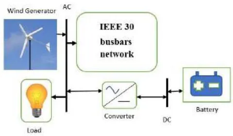
This paper examines the possibility of using wind power energy for electricity generation at optimum conditions and simulation network for an IEEE 30 -buses, which consists of 30 busbars was connected via 38 transmission lines, is considered for this study. The objectives are to identify more economic technology and the environmental merit of the wind microgrid.
The estimated electrical real power generation of 300 MW while the valued electrical load The consumption of 285 MW. A MATLAB program was used to analyze the system they allow comparison with different design options.
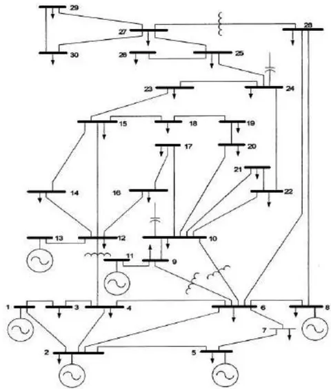
The proposed technique is performed and verified on the IEEE 30 busbars network. The power system network construction of 30-buses was indicated in Figure 1. In this network, there are 6-generators in the system, one on the bus slack and the other on the buses 2,5,8,11, and 13 respectively. There are 4-tap changer transformers between buses (4,12), (6,9), (6,10), and (27.28). There are 2-synchronous capacitors on bus 10, and bus 24 respectively.
VII. Technical specifications E-126 ENERCON wind energy converters
ENERCON wind energy converters run with a special storm control feature. A slows the wind turbine down so that it can continue to operate even at high wind speeds. Numerous shutdowns which lead to considerable losses in power output can thus be avoided. In this paper connected A E-126 ENERCON wind energy converters as DG with specifications given in table 1. Figure 2 illustrates Power-Wind speed characteristics for 7.5 MW /E-126 ENERCON wind energy converters, while Figure 3 shows the characteristics of Power Coefficient-Wind speed for it's.
| Rated power | 7500 kW |
| diameter of Rotor | 127 m |
| Hub height | 135 m |
| blades No. | 3 |
| The swept area in m2 | 12,668 |
| Rotational speed | Variable, 5 - 12.1 rpm |
| Cut-out wind speed: (with ENERCON storm control*) | 28 - 34 m/s |
{"image_source":{"path":"images/e85a3fe50aa94bcb0db833807164244bea3dd35525668f9089d477889ebd56ed.jpg"},"content":"","chart_caption":[{"type":"text","content":"Figure 2: Power-Wind speed characteristics"}],"chart_footnote":[]} {"image_source":{"path":"images/0486adf8392530cccc57264aff9c66f1ec98d98bff4a8c6f8b99e9639d454c1b.jpg"},"content":"","chart_caption":[],"chart_footnote":[]}
VIII. SELECTION PARTICLES OF PSO AND APSO
In this paper, the particle selected in each technique as the voltage magnitude at slack bus and each P|V| generation bus, also tap changing transformer ratio and the injected reactive power to the system. So there are 12 different particles are ( , , , , , ) form slack and P|V | magnitude voltages, tap changing transformer ratio ( , , , ) between buses 4-12, 6-9, 6-10, and 27-28 and injected reactive power ( , ) at buses 10 and 24. When the optimization development process begins, each particle position will be a continuous update until reach the stop criteria.
The minimum inertia weight was selected as 0.45, and the maximum weight limitations were selected as 0.95. With continuous repetition, the weight value will drop from 0.95 to 0.45.
XI. RESULTS AND DISCUSSION
In this section, we show all the results obtained from running the MATLAB program for standard PSO and APSO techniques:
Figure 5 shows the process of optimizing interactive power transmission with Installation of wind generator at the optimum location of bus no. 24, for the PSO technique, when the optimization is starting development, the position of the particles are chosen arbitrarily. The global real optimum power loss is 16.58 MW, then the particles constantly update their attitudes towards the better solution, the loss of active power remains to decline. Later 45 iterations, there can be no clear upgrading observed. Finally, the loss of real power is close to 15.15 MW.
Also, figure 6 illustrates the optimizing process interactive power transmission with Installation of wind generator at the optimum location of bus no. 15, for the APSO technique, at the starting of the optimization, the particles locations are chosen arbitrarily. The loss of active power is about 14.1 MW. When the particles update their attitudes towards the best solution, also the loss of real power remains to decline, and after 2 iterations, the loss of active power is close to 13.69 MW.
Figure 7 shows the actual power loss per branch before and after installed DG at the optimum location by using PSO and APSO techniques. This figure illustrates the loss of active power in most lines slightly decrease, (as branches from 1 to 6) when using APSO technique so the total real power loss of 30 the bus system was greatly reduced and the higher losses in each branch when using PSO without wind turbine generator.
Figures 8 and 9 show the power losses when installing the wind generator located in a different position of the bus then it shows the minimum power, where for case PSO technique the minimum power accord when the DG located at bus 15 and the power losses of 15.15MW, And for case APSO technique the minimum power accord when the DG was located at bus 24 and the power losses of 13.157MW. So, this illustrates that the power losses reduce when using APSO technique, Figure 10 shows the difference in power losses when installing the wind generator located in a different location of the bus when using PSO and APSO techniques.
{"image_source":{"path":"images/cb9fa3918f550f6801f465b36fc5cf5866a5a2bc8b8c07ab8df5c21bb5d8ef2e.jpg"},"content":"","chart_caption":[{"type":"text","content":"Figure 5: Minimum power losses when using PSO technique"}],"chart_footnote":[]} {"image_source":{"path":"images/6b3aee65498f3cb691b870f5808b92cab132b64debf3d14f71c3dbe132735d81.jpg"},"content":"","chart_caption":[{"type":"text","content":"Figure 6: Minimum power losses when using APSO technique"}],"chart_footnote":[]}
{"image_source":{"path":"images/f63fe1056867f55ba2adbb5694481d7016ab621d876193e0c34e63296a37de66.jpg"},"content":"","chart_caption":[],"chart_footnote":[]} {"image_source":{"path":"images/a4a031de2decac7f895b0bfac031478a8c96246ead91fcd71a203428f334bc28.jpg"},"content":"","chart_caption":[{"type":"text","content":"Figure 7: The Real Power Loss at Each Branch"}],"chart_footnote":[]}
{"image_source":{"path":"images/e949e445a07cffcafffe809d0548d2f01360423e186bcd8827d5bb5651ab9b89.jpg"},"content":"","chart_caption":[{"type":"text","content":"Figure 8: Active power losses when using the PSO technique when location DG at different busses"},{"type":"text","content":"Figure 9: Active power losses when using the APSO technique when location DG at different busses"}],"chart_footnote":[]} {"image_source":{"path":"images/a81d4435d7932b7b322ecabc27dbcb8e5e27f8ca76766d6ba4528ca7483318df.jpg"},"content":"","chart_caption":[{"type":"text","content":"Figure 10: Active power losses comparison when using PSO and APSO technique when location DG at different busses"}],"chart_footnote":[]}
The voltage profile was evaluated using The Fast-Decoupled Load Flow (FDLF) method then calculate the real power loss of the system. After that put wind generator at each bus to estimate the total corresponding real power losses to obtain the optimal location of the DG when the total loss accord. This paper provides a new technique proposed solution to determine the optimal location of the DG in the power system. The proposed approach is based on the APSO technique and aims at the identification of the position of the load is different and compare the results with the applied standard PSO technique. Figure 11 shows the magnitude voltage profile for different cases for PSO and APSO techniques with and without, the figure illustrates the voltage magnitude will be improved when using APSO with an installed wind generator. Also, Figure 12 explain the voltage phase angle also modified.
{"image_source":{"path":"images/d9458f397787e05cc45a0f18b3cefde668bb277986ee6f40840c655b91234602.jpg"},"content":"","chart_caption":[{"type":"text","content":"Figure 11: Voltage magnitude profile"}],"chart_footnote":[]} {"image_source":{"path":"images/a594dad190e2a9e16e332a9a1bac1a436278f4449810275b0d4f9b12fb9a4045.jpg"},"content":"","chart_caption":[{"type":"text","content":"Figure 12: Voltage angle profile"}],"chart_footnote":[]}
X. CONCLUSIONS
In this paper, the comparison between two techniques are used to identification of an optimum location by using standard particle swarm optimization technique and accelerated particle swarm optimization technique; the obtained results explain the affiant the APSO method when taking the consideration of iteration number, fast of execution time, reducing power losses, improve the power losses on the transmission line and optimize the power flow, and improve the magnitude and angle voltage profile.
Conflict of Interest
The authors declare no conflict of interest.
Ethical Approval
Not applicable
Data Availability
The datasets used in this study are openly available at [repository link] and the source code is available on GitHub at [GitHub link].
Funding
This work did not receive any external funding.
References
Cite this article
Related Research


Special Issue
Launch a focused special issue to highlight research, emerging trends, and expert insights in your academic field.