

IntelliPaper
Abstract
It is known that the fluid or gas laminar flow velocity spontaneous increase (without external forces) leads
to a turbulent flow [1]. The mechanism of flow spontaneous change from laminar to turbulent is not found.
Obviously, a source of forces perpendicular to flow velocity must be detected.
Further, it is shown that the fluid moving masses gravitomagnetic interaction may be the cause of
turbulence.
Explore Digital Article Text
I. INTRODUCTION
It is known that the fluid or gas laminar flow velocity spontaneous increase (without external forces) leads to a turbulent flow . The mechanism of flow spontaneous change from laminar to turbulent is not found. Obviously, a source of forces perpendicular to flow velocity must be detected.
Further, it is shown that the fluid moving masses gravitomagnetic interaction may be the cause of turbulence.
In , the mechanism of the appearance of turbulent flows is considered and an approach to the method for calculating such flows is indicated. In , a new method for the numerical solution of the Navier-Stokes equation is proposed. At the beginning of the article, this method is briefly described and an example is given of calculating the flow in a mixer. Further, this method extends to the calculation of stationary flows with turbulence. An algorithm for this calculation is also proposed, and an example is given of calculating the flow in a mixer with turbulence.
It is shown in that there are forces of interaction between moving masses. These forces depend on the mass, velocity, and distance between masses. It was shown in that groups of molecules forming the element of the jet interact in a similar way. In particular, when the velocity vectors of the jets are equal and the masses of the groups are equal , the force of the interaction between these groups is determined by the formula
where r is distance between groups,
d is characteristic size of the group,
is density of the liquid,
is coefficient of gravity permeability of vacuum [3].
, which follows from general relativity, c is speed of light in vacuum, cm·s ;
is gravitational constant, .
On this basis further in it is shown that turbulent forces arise in the liquid. In this case, the force acting on the unit volume,
where the operator, which hereinafter for brevity sake will be called as turbulean,
turbulent density of a given fluid
It can be seen that the turbulent force has the dimension of the mass force acting per unit volume. Therefore, the turbulent forces (2) can be included in the Navier-Stokes equations. The Navier-Stokes equations supplemented by such forces become equations of hydrodynamics for turbulent flow.
These equations have the form:
where p is the pressure. In the stationary regime, equation (6) takes the formrge p - давление.
It was shown in [2] that instead of equation (7) a modified equation can be considered, which has the following form:
where the quasipressure
In this case
Here
In [2] it is shown that in the flow of a viscous incompressible fluid there is a power balance:
where the power of mass forces
power of mass forces
power of the change in the energy loss by internal friction during motion
power of changing the energy flow through a given volume of liquid
power of the change in energy as the direction of the flow changes
power of change of work of pressures
From (16, 17) we find:
Finally, from (11, 19) we obtain:
II. THE SOLUTION OF THE MODIFIED NAVIER-STOKES EQUATIONS
First we consider the modified Navier-Stokes equations without turbulent forces:
where are unknown , . Following [2], to solve this system of equations, we consider the functional
is a constant. The gradient of this functional has the form
Where
It was shown in [2] that the functional (3) is convex and the minimum of the functional (3), achieved when the gradient (5) is zero, i.e. when
always exists and is unique and global. Consequently, the minimization of the functional (3) by moving along the gradient (5) is equivalent to solving the equation (7) with unknowns v
It was shown in [2] that
Thus, simultaneously with the minimization of the divergence , there is defined an that satisfies the equation (7). By increasing the value , it is possible to achieve arbitrarily high accuracy of solving equations (2). Consequently, the minimization of the functional (3) by moving along the gradient (5) is equivalent for at sufficiently large r solution of the system of modified equations (1, 2) with unknowns v, D, i.e. reduces to finding the minimum of a convex functional
After solving the system of equations , the pressure is calculated from equation
which follows from (1.11). In this case (1.20) takes the form:
The algorithm for the motion along the gradient (5) of the functional (3) has the following form: 1. We consider the gradient (5)
where Q is the three-dimensional region of flow existence, and all variables are three-dimensional vectors (in the sense of vector algebra). Here and below multiplication by Q means that the vectors of those points that are not in the region Q are zeroed. Further, the multiplication sign, if it refers to vectors, means the componentwise multiplication of vectors.
- Zero values of all velocities in the region are considered. Q.
3. Coefficients are calculated:
4. New velocity values are calculated:
(11)
- The criterion for stopping the calculation is checked and, if it is not fulfilled, the transition to step 3 is performed. The stopping criterion can be the achievement of a power balance (see also (1.12)
III. AN EXAMPLE OF A SOLUTION OF A STATIONARY PROBLEM
Let us consider a mixer, whose lades are made of fine-mesh material and are located close enough to one another. Then the pressure forces of the blades on the fluid may be equated to body forces. Let us assume that the body forces created by mixer's blades and acting along a circle with its center in the coordinate origin, are described as follows {"image_source":{"path":"images/f00128de64c1237fa47f2f67d33b3167e5c5fcc6a97ebbcb39acd42929092952.jpg"},"content":"","chart_caption":[],"chart_footnote":[]}
{"image_source":{"path":"images/3f72dbc953c8df99d2a42a9cbc75a78be889e280fcbee901b8490fb3cb7c53a8.jpg"},"content":"","chart_caption":[],"chart_footnote":[]}
Let us assume that the body forces created by mixer's blades and acting along a circle with its center in the coordinate origin, are described as follows
where
(1)
R is the distance from the current point to the rotation axis,
are certain constants.
For , the function (1) is shown in Fig. 1, and gradient of forces (1) is shown on Fig.
The projections of forces (1) on the axis of Cartesian coordinates have the form
Next, consider a mixer with a cylindrical wall located on a circle of radius . These walls create a closed system and do not change the power balance in the system. The region of integration is limited to a circle with a radius . It is important to note that on the circle of radius the speed is v = 0. This answers the known fact that due to vicious friction the speed of fluid on the surface of a body surrounding it, is equal to zero. It is also important to note that to get this result we had not have to add more equations in the main equation - it was enough to restrict the integration domain.
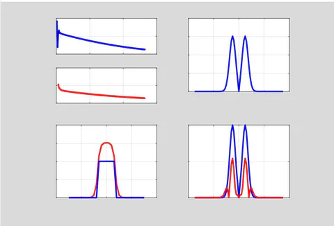
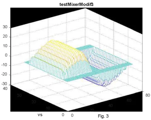
The conditions of the computational problem are indicated in detail in [2]. In Fig. 3 shows some graphs:
Relative error in calculating speed - see the first window on the first vertical;
Relative error in calculating divergence of speed - see the second window on the first vertical;
Speed function as a function of the radius - see the first window on the second vertical;
Speed function , depending on the height distance to the center of the mixer with a constant radius value - see the third window on the first vertical; rectangle in this window indicates area of act force;
Function of force and the Lagrangian function as a function of the radius - see the fourth window, where the function has a larger value of the maximum
Method and Algorithm for Calculation of Turbulent Flows {"image_source":{"path":"images/8adc0ad176f9c3a9ddc18ff45b73b2ae754856bf66ee89f2e796ed196a9cad72.jpg"},"content":"","chart_caption":[{"type":"text","content":"Fig. 5."}],"chart_footnote":[]}
We denote by the velocity along the horizontal circle. In Fig. 4 shows the diagram of this velocity on a vertical plane passing through the axis oy. In Fig. 5 shows the diagram of this velocity in the horizontal plane passing through the middle of the mixer.
IV. SOLUTION OF MODIFIED NAVIER-STOKES EQUATIONS WITH TURBULENCE
In this case, it is necessary to solve the system of equations (1.5, 1.7). However, this functional (as for the equations (2.1, 2.2)) is not convex and, consequently, its minimization can not be performed by moving along the gradient. Therefore, let us consider another method for solving the system of equations (1.5, 1.7).
Turbulent flow with limited turbulence can be regarded as the sum of two processes:
laminar flow with "trunk speeds", caused by mass forces ,
turbulence with "additional speeds" caused by forces .
At the same time, the "trunk speeds" of the flow are not changed by forces , but these forces create "additional speeds" that cause the flow elements to oscillate relative to the "main direction". These additional speeds are much smaller than the trunk speeds. Under this assumption, the algorithm for solving the system of equations (1.5, 1.7) can be as follows:
We accept . In this case, the system of equations (1.5, 1.7) takes the form (2.1, 2.2).
We solve the system of equations (2.1, 2.2) by the algorithm described in Section 2, and determine the backbone speeds and the corresponding quasi-pressures .
We calculate the powers , , . These powers are determined by (1.13, 1.15, 1.16), respectively. In this case, the power balance condition must be satisfied.
At known speeds we find the forces according to (1.2).
5. Solve a system of equations of the form
This system of equations formally coincides with the system of equations (2.1, 2.2) and is also solved by the algorithm described in Section 2. In this case, the speeds caused by forces and the corresponding quasi-pressures are determined.
{"image_source":{"path":"images/aaf89b700ed84a52e8c71b548cd6ca5261bc2d34a228e94d43c8fec7a60e8057.jpg"},"content":"","chart_caption":[],"chart_footnote":[]}
We calculate the powers , , according to (1.13, 1.15, 1.16). In this case, the condition must be satisfied. Here is simultaneously the power of the turbulent forces.
Total capacities , , . are found as the sum of the capacities found in points 3 and 6.
Determine the total speeds and total quasi-pressures .
By (1.10), we determine the pressure p.
V. AN EXAMPLE OF THE SOLUTION OF THE PROBLEM WITH TURBULENCE
Again, consider the flow in the mixer - as in Section 3.
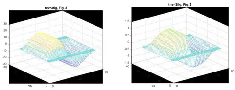
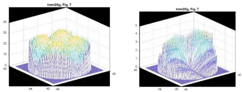
Various graphs are given below, with the left figures referring to the calculation by clause 3, and the right drawings refer to the calculation by clause 6 for .
In Fig. 6 shows the errors of the execution of equations (2.2) and 2.1) depending on the number of iterations - see Error1 and Error2, respectively.
In Fig. 7 shows the speed as functions of the radius.
In Fig. 8 shows the speed as a function of the height distance to the center of the mixer for a constant value of radius; a rectangle in this window indicates the range of force.
In Fig. 9 shows the force and Lagrangian as a function of the radius, where value of maximum for force have a larger value of maximum for Lagrangian .
We denote by the velocity along the horizontal circle.
In Fig. 10 shows the diagrams of this velocity on the vertical plane passing through the axis oy.
In Fig. 11 shows the velocity diagrams in the horizontal plane of the plane passing through the middle of the mixer.
{"image_source":{"path":"images/a56eac30154866b47b129ff83331e72adaa9a2534934e7141c38f61ded009f37.jpg"},"content":"","chart_caption":[{"type":"text","content":"Fig. 6."}],"chart_footnote":[]} {"image_source":{"path":"images/4da10a6963040712a7bedf0c5589fa14dbe6f8f0918101ad50a287add1e1200c.jpg"},"content":"","chart_caption":[],"chart_footnote":[]}
{"image_source":{"path":"images/1a5d29b04d524fb592824838b6d2a2e7f5c140d9f602be4c5ada59132d351bcd.jpg"},"content":"","chart_caption":[{"type":"text","content":"Fig. 7."}],"chart_footnote":[{"type":"text","content":"Method and Algorithm for Calculation of Turbulent Flows"}]}
{"image_source":{"path":"images/3a50dfa01de23b8cf8ad90f0325a8a1eeb279454f7324c05b91b04bb0576570b.jpg"},"content":"","chart_caption":[],"chart_footnote":[]} {"image_source":{"path":"images/723c1bb3c85701fad7f76bdfdbda977a7f47bb5e1eff963e2cea802e326c0530.jpg"},"content":"","chart_caption":[{"type":"text","content":"Fig. 8."}],"chart_footnote":[]}
{"image_source":{"path":"images/04e004063a4f41a1659a954c0d267afe1caad2ed9278d58cadeac68689969df5.jpg"},"content":"","chart_caption":[],"chart_footnote":[]} {"image_source":{"path":"images/62e3be6e9997af0ff5b6110ed363870124a44da4183ca265d163697dab20f731.jpg"},"content":"","chart_caption":[{"type":"text","content":"Fig. 9."}],"chart_footnote":[]}
The initial data and the results of the calculation are summarized in Table.
Column 3 of this table shows the results of solving the system of equations (5.2) in accordance with p. 2 of the algorithm under consideration.
Columns 4 and 5 of this table show the results of solving the system of equations (10, 11) with p. 5 of the algorithm under consideration.
Table 1.
| Notation | Dimension | Parameters | Without turbulence | With turbulence | With turbulence |
| 1 | 2 | 3 | 4 | 5 | |
| Turbulent density | 0 | 10 | 1 | ||
| ρ | Density of a liquid | 1.7 | 1.7 | 1.7 | |
| μ | Coefficient of internal friction | 0.7 | 0.7 | 0.7 | |
| k | Number of iterations | 1500 | 500 | 500 | |
| r | Parameter | 100 | 100 | 100 | |
| ε | Relative error in the fulfillment of the equations of hydrodynamics | ||||
| Thermal power | |||||
| Power of mass forces | |||||
| Power change in energy flow | |||||
| Power imbalance | |||||
| Relative power imbalance | 0.0128 | 0.0191 | 0.0191 | ||
| Total power of the mass forces | |||||
| Coefficient of efficiency | 1 | 1.76 | 1.0076 | ||
| mid(ν) | Mean square speed | 9.49 | 4.54 | 0.45 | |
| mid(∇D) | Mean square quasi-pressure gradient | 0.0389 | 0.0453 | 0.0143 | |
| div | Mean square divergence at a point | 0.452 | 0.613 | 0.0614 | |
| mid(F) | Mean square mass force | 0.947 | 1.865 | 0.186 |
It can be noted that
For a certain number of iterations, the power balance equation is fulfilled - see the line «Relative power imbalance», where .
The additional speeds V shown in the "root mean square speed" line and columns 4-5 are significantly smaller than the trunk speeds Vo shown in the same row and column 3. Here, too, we see that V << Vo. Hence our assumption is fulfilled.
At the same time, the error in the execution of the system of equations (5.2) and the system of equations (10, 11) also becomes insignificant - see the line "Relative error...". This value is calculated by the formula .
At the same time, the error in executing the equation div = 0 also becomes insignificant - see the line "Mean square divergence".
It can be seen in Table 1 and Fig. 1-7, that when additional turbulent forces are taken into account, additional powers and appear, i.e. the energy of turbulent forces is converted into energy of heating and work of pressures - turbulence raises temperature and pressure.
Exceeding the power of mass forces due to additional turbulent forces we will estimate the efficiency coefficient .
VI. CONCLUSIONS
Turbulence is caused by the gravitational field of the Earth. The forces of turbulence and the kinetic energy of turbulent motion can be calculated from the equations of hydrodynamics supplemented by turbulean.
The influence of gravitomagnetic forces increases with the speed of motion. Therefore, at low speeds a laminar flow is observed, but turbulent forces play an important role with increasing speed. An anonymous author in formulates a very profound observation:
Traditional hydrodynamics tacitly based on axiom that the true mode of fluids and gases motion is a laminar current, and turbulence is regarded as its violation caused by a particular restriction of its "freedom". However, based on the fact that the current that was laminar in a relatively narrow channel, when removing the walls that limit it and remaining the previous velocity begins to swirl, it is logical to conclude that exactly vortex flow is a "natural" mode of fluids and gases motion, and it becomes forcedly laminar - just under the influence of environmental constraints! It is enough to look at Reynolds number formula - generally accepted criterion of flow laminarity or turbulence - in case of constant flow rate it increases proportionally to pipe diameter, which means that the current becomes more turbulent. A fluid whirling at a high velocity in a narrow tube is laminar, and even slow currents in the limitless ocean are accompanied by rotary streams and vortices - the same slow, low-observable and safe as flows that have generated them.
There are devices in which this additional energy generated by turbulent forces is used - so-called cavitation heat generators. The first such device was "Apparatus for Heating Fluids" by J. Griggs [5]. In it "the rotor rides a shaft which is driven by external power means. Fluid injected into the device is subjected to relative motion between the rotor and the device housing, and exits the device at increased pressure and/or temperature". At present, there are many such devices that differ in the ways of creating turbulent motion - see, for example, [6], where there are also references to many prototypes. Such devices provide efficient, simply, inexpensive and reliable sources of heated water and other fluids for residential and industrial use.
Together with the existence of cavitation heat generators there is no generally accepted theory that reveals the source of additional energy that appears as a result of the functioning of these cavitation heat generators. In particular, Griggs in [5] points out that his "device is 6 thermodynamically highly efficient, despite the structural and mechanical simplicity of the rotor and other compounds", but does not provide a theoretical justification for this statement. The authors of the following devices also do not consider the reasons for the efficiency of their devices.
The application of the proposed method for calculating turbulent flows allows for optimal design of such devices.
There are other devices demonstrating the existence of an inexplicable increase in energy, for example, Rank's tube , Kotousov's nozzle . For them, there is also no calculation method and the proposed method can be applied.
Annotation
An algorithm for calculating turbulent flows is described. Examples of calculation are given. It is noted that the proposed algorithm can be used to calculate and optimize cavitation heaters.
Conflict of Interest
The authors declare no conflict of interest.
Ethical Approval
Not applicable
Data Availability
The datasets used in this study are openly available at [repository link] and the source code is available on GitHub at [GitHub link].
Funding
This work did not receive any external funding.
References
Cite this article
Related Research

Special Issue
Launch a focused special issue to highlight research, emerging trends, and expert insights in your academic field.