





IntelliPaper
Abstract
Repeatedly, the Brazilian Judicial System has determined that home-financing contracts written in terms of compound interest, both in the case of constant payments and in the case of the system of constant amortization, should be substituted by contracts specifying simple interest. This has resulted, for the case of the system of constant mortization, in the adoption of a variant of a procedure that has been named the “Gauss’ Method”. It is shown that the implementation of a multiple contracts’ version may imply substantial fiscal gains, depending on the financial institution opportunity cost.
Explore Digital Article Text
I. INTRODUCTION
Similar to the case of constant payments, which in terms of multiple contracts, was recently analyzed in de Faro and Lachtermacher (2023), the Brazilian Judicial System, cf. Jusbrasil (2023), has repeatedly determined that the System of Constant Amortization (SAC, with the acronym as written in Portuguese), which was introduced in the Brazilian System of House Financing (SFH) in 1971, and which is based on compound interest, should also be substituted by a version based on simple interest.
For this purpose, Rovina (2009) proposed a variant of the so called "Gauss' Method," cf. Nogueira (2013), to consider that in the system of constant amortization, the periodic payments follow an arithmetic progression.
Although promulgated in several sentences, the above-mentioned procedure violates a law established in 1964. For this reason, besides considering the afore-mentioned variant of the so called "Gauss' Method," which considers the end of the contract as the focal date, cf. Ayres (1963), we will also consider the case where the focal date, complying with the 1964 law, specifies the beginning of the contract as the focal date.
II. THE ROVINA'S PROPOSAL
Consider a house-financing contract of F units of capital, with terms of n periods, specifying the periodic rate i of compound interest, in accordance with the system of constant amortization.
Denoting by the k-th payment, it can be seen, for instance in de Faro and Lachtermacher (2012, p.267), that we will have:
That is, the periodic payments will follow an arithmetic progression, with initial payment and negative ratio equal to .
Consequently, the outstanding debt at the end of the -th period, just after the -th payment, denoted , will linearly decrease. That is:
with .
On the other hand, in the case where the interest rate, i, is of simple interest, we must specify a particular focal date.
In general, if the end of the contract is specified as the focal date, denoting by the k-th periodic payment, we must have:
According with Rovina (2009), who extended the so called "Gauss' Method," as in Nogueira (2013), to the case where the periodic payments follow an arithmetic progression, the first step is to introduce a weight factor, I, defined as:
Consequently, the k-th periodic payment will be:
That is, the periodic payments follow an arithmetic progression with first payment and with ratio , which can be shown to satisfy equation (2).
Furthermore, as in the SAC with compound interest, we will have constant amortization, with the k-th parcel of interest, , being made equal to:
As shown in de Faro (2014), we have , if . Therefore, the recipient of the loan is always benefited if the contract originally written in terms of compound interest, is substituted by one, at the same rate i, written in terms of simple interest.
Before proceeding, it should be noted, as pointed out by De-Losso et al. (2020), that the specification of the end term of the contract as the focal date, violates a Brazilian law of 1964, which stipulates that the focal date must be the beginning of the contract. This point will be further addressed in section 6.
Notwithstanding, although this peculiar variant of the "Gauss' Method" is plagued by several financial deficiencies, as discussed in de Faro (2014), it is still being judicially supported.
III. A SIMPLE NUMERICAL EXAMPLE
Fixing at 1% the periodic interest rate, i, of simple interest, consider a loan of 10,000 units of capital with a single contract specifying 12 periodic payments in accordance with this variant of the "Gauss' Method." The weight factor, I, in this case is equal to 7.76397516.
In Table 1, using formulas (4) and (5), and the fact that the parcel of amortization is constant, we present the evolution of the debt , as given, recursively, as with . Consequently, as in the case where i is a rate of compound interest, also decreases linearly.
Table 1: Evolution of the Debt According with the Rovina's Variant of the "Gauss' Method" – Focal Date = n
| k | $J_k$ | $A_k$ | $P_k$ | $S_k$ |
| 0 | 10,000.00 | |||
| 1 | 93.17 | 833.33 | 926.50 | 9,166.67 |
| 2 | 85.40 | 833.33 | 918.74 | 8,333.33 |
| 3 | 77.64 | 833.33 | 910.97 | 7,500.00 |
| 4 | 69.88 | 833.33 | 903.21 | 6,666.67 |
| 5 | 62.11 | 833.33 | 895.45 | 5,833.33 |
| 6 | 54.35 | 833.33 | 887.68 | 5,000.00 |
| 7 | 46.58 | 833.33 | 879.92 | 4,166.67 |
| 8 | 38.82 | 833.33 | 872.15 | 3,333.33 |
| 9 | 31.06 | 833.33 | 864.39 | 2,500.00 |
| 10 | 23.29 | 833.33 | 856.63 | 1,666.67 |
| 11 | 15.53 | 833.33 | 848.86 | 833.33 |
| 12 | 7.76 | 833.33 | 841.10 | 0.00 |
| Σ | 605.59 | 10,000.00 | 10,605.59 |
Before proceeding, it is imperative to point out that the determination of the outstanding debt at time k, , as given by the recursion mentioned above, does not agree with the results that would be derived by the well-established concepts of either the retrospective method or by the prospective method, which, following Kellison (1991), states that:
a) according to the prospective method, the outstanding loan balance at any point in time is equal to the present value on the date of the remaining payments.
For instance, at time 10, just after the payment, as we are using simple interest, we would have:
units of capital;
while, according to Table 1 we would have units of capital.
According to the retrospective method, the outstanding loan balance at any point in time is equal to the original amount of the loan accumulated to that date less the accumulated value on the date of all payments previously made.
Thus, for instance, the outstanding loan balance just after the second payment, would have to be:
On the other hand, the results presented in Table 1 would imply that units of capital.
To remedy this incongruence, which may result in judicial arguments, Lachtermacher and de Faro (2023) extended the work of Forger (2009) providing a financially consistent procedure. This point will be further addressed in section 6.
However, given that the parcels of interest are not affected, we will proceed with the analysis accordingly.
IV. IMPLEMENTING MULTIPLE CONTRACTS
Rather than engaging in a single contract, the financial institution has the option of requiring the borrower to adhere to n subcontracts - one for each of the n payments that would be associated with the case of a single contract.
If the rate i were of compound interest, the principal of the k-th subcontract, as proposed in De-Losso et al. (2013), in what can be deemed as an adaptation of the master thesis of Sandrini (2007), the principal of the k-th subcontract would be taken to be equal to the present value of the k-th payment of the original single contract – a procedure that was also used in de Faro (2022) and in de Faro and Lachtermacher (2023 a and b).
However, as we are considering the case where the rate i is of simple interest, and the focal date is taken to be the end of the contract, we must make an adaptation, which was suggested in Lachtermacher and de Faro (2023). In this case, the principal of the k-th subcontract, denoted as , will be:
In this manner we are assured that the sum of the principal of the n subcontracts will be exactly equal to the principal F of the original single contract.
As for the component of amortization that is associated with the k-th subcontract, we will have:
On the other hand, and this is the key factor which justifies the financing institution's gain for substituting a single contract by subcontracts, the component of interest, associated with the -th subcontract, denoted as , will now be:
Therefore, considering our simple numerical example of section 3, Table 2 presents the sequence of the 12 constant payments, which is the same in both the case of a single contract, as well in the case of the 12 individual subcontracts.
Additionally, Table 2 also presents the sequences and , as well as the sequence of differences .
As previously pointed out, it should be noted that the original debt of 10,000 units of capital is fully amortized, since:
in this case with .
Formally, however, we do not have a system of constant amortization anymore as the parcels of amortization are not equal.
Table 2: The Sequences of the Parcels of Interest and its Differences (Focal Date = n)
| Multiple Contracts | |||||
| k | $F_k$ | $\overline{A}_k$ | $\overline{J}_k$ | $P_k$ | $d_k$ |
| 1 | 918.23 | 918.23 | 8.27 | 926.50 | 84.90 |
| 2 | 902.33 | 902.33 | 16.41 | 918.74 | 69.00 |
| 3 | 886.57 | 886.57 | 24.40 | 910.97 | 53.24 |
| 4 | 870.95 | 870.95 | 32.26 | 903.21 | 37.62 |
| 5 | 855.47 | 855.47 | 39.98 | 895.45 | 22.14 |
| 6 | 840.92 | 840.92 | 47.55 | 887.68 | 6.79 |
| 7 | 824.92 | 824.92 | 54.99 | 879.92 | -8.41 |
| 8 | 809.86 | 809.86 | 62.30 | 872.15 | -23.48 |
| 9 | 794.93 | 794.93 | 69.46 | 864.39 | -38.40 |
| 10 | 780.14 | 780.14 | 76.48 | 856.63 | -53.19 |
| 11 | 765.49 | 765.49 | 83.37 | 848.86 | -67.84 |
| 12 | 750.98 | 750.98 | 90.12 | 841.10 | -82.35 |
| Σ | 10,000.00 | 605.59 | 10,605.59 | 0,00 | |
Strictly from an accounting point of view, there is no gain for the financial institution granting the loan if a single contract is substituted by multiple contracts, since the sums of the corresponding parcels of interest is the same. That is:
Yet, depending on the opportunity cost of the financial institution, which will be denoted as , and is usually of compound interest, and which is supposed to be relative to the same period of the simple interest rate, i, that is being charged, the financial institution may derive substantial gains in terms of tax deductions.
In other words, it is possible that:
where denotes the present value, at the rate of the sequence of the parcels of interest in the case of a single contract, and denotes the corresponding present value in the case of the adoption of multiple contracts.
Moreover, at least in the case of our simple numerical example, as the sequence of differences has only one change of sign, thus characterizing what is termed a conventional financing project, cf. de Faro (1974), whose internal rate of return is unique, and in this particular case is null, it follows that if .
Figure 1 outlines the evolution of , for per period, for units of capital and . Additionally, we also have the evolution of , where the simple interest rate, , is equal to , , , , and per period.
{"image_source":{"path":"images/7fc9df4d360a9cd54d2111de22e027a8e43909617a73d313aca160a7cb105adc.jpg"},"content":"","chart_caption":[{"type":"text","content":"Figure 1: Values of "},{"type":"equation_inline","content":"\Delta"},{"type":"text","content":", F=10,000 units of capital and n=12"}],"chart_footnote":[]}
V. GENERAL ANALYSIS - DATA FOCAL AT TIME N
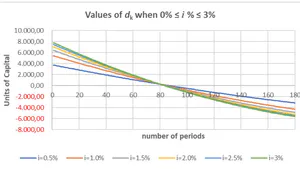
In the previous section, focusing attention on our simple example, with only 12 periods, it was verified that the sequence of differences of the interest payments present just one change of sign, thereby assuring us of the uniqueness of the corresponding internal rate of return, which is known to be null.
Furthermore, this inference appears to always be true, as supported by the evidence provided in Figure 2, which presents the evolution of the sequence for the case where F = 1, 200, 000 units of capital of a single contract with 180 periods and with the simple interest rate, i, being as high as 3% per period.
{"image_source":{"path":"images/d11b3fa5b224018ba2c6396fd0afe7d48f583479076fe78ae84b730fd3ab7559.jpg"},"content":"","chart_caption":[{"type":"text","content":"Figure 2: Values of "},{"type":"equationinline","content":"d\{k}"},{"type":"text","content":", F=1,200,000 units of capital and n=180."}],"chart_footnote":[]}
Consequently, it can be inferred that the financing institution is always better off if a single contract is substituted by multiple contracts - one for each one of the n payments of the original contract.
Taking into account that in Brazil the monthly interest rates charged do not exceed 2% per month, in real terms, we are going to analyze the behavior of the percentage increase of the fiscal gain for some values of the corresponding annual opportunity cost , with each contract with a term of years.
Table 3: Fiscal gain , the end term of the contract as the focal date, .
| $\rho_a(\%)$ | ||||||
| $n_a$ | 5% | 10% | 15% | 20% | 25% | 30% |
| 5 | 7.9719 | 16.1314 | 24.4507 | 32.9031 | 41.4632 | 50.1072 |
| 10 | 16.2389 | 33.9052 | 52.8273 | 72.8069 | 93.6337 | 115.0988 |
| 15 | 24.8052 | 53.2265 | 84.7246 | 118.6077 | 154.1421 | 190.6437 |
| 20 | 33.7337 | 74.1080 | 119.7820 | 169.0355 | 220.2051 | 271.9532 |
| 25 | 43.0539 | 96.4714 | 157.4421 | 222.6120 | 289.1879 | 355.3285 |
| 30 | 52.7773 | 120.1807 | 197.0807 | 278.0298 | 359.2563 | 438.7897 |
Table 4: Fiscal gain
, the end term of the contract as the focal date, .
| $\rho_a(\%)$ | ||||||
| $n_a$ | 5% | 10% | 15% | 20% | 25% | 30% |
| 5 | 7.7552 | 15.6718 | 23.7228 | 31.8826 | 40.1269 | 48.4330 |
| 10 | 15.6890 | 32.6551 | 50.7238 | 69.7007 | 89.3852 | 109.5827 |
| 15 | 23.9269 | 51.1075 | 80.9942 | 112.9219 | 146.2102 | 180.2417 |
| 20 | 32.5457 | 71.0942 | 114.3113 | 160.5803 | 208.3928 | 256.5663 |
| 25 | 41.5726 | 92.5563 | 150.2096 | 211.4310 | 273.7177 | 335.4564 |
| 30 | 51.0157 | 115.3712 | 188.1381 | 264.3247 | 340.5672 | 415.1392 |
Table 5: Fiscal gain
, the end term of the contract as the focal date, .
| $\rho_a(\%)$ | ||||||
| $n_a$ | 5% | 10% | 15% | 20% | 25% | 30% |
| 5 | 7.6074 | 15.3594 | 23.2297 | 31.1934 | 39.2270 | 47.3088 |
| 10 | 15.3771 | 31.9511 | 49.5475 | 67.9753 | 87.0402 | 106.5558 |
| 15 | 23.4807 | 50.0420 | 79.1365 | 110.1156 | 142.3264 | 175.1843 |
| 20 | 31.9849 | 69.6895 | 111.7900 | 156.7216 | 203.0461 | 249.6486 |
| 25 | 40.9094 | 90.8278 | 147.0548 | 206.6009 | 267.0851 | 326.9859 |
| 30 | 50.2576 | 113.3324 | 184.3928 | 258.6363 | 332.8607 | 405.4327 |
Table 6: Fiscal gain
, the end term of the contract as the focal date, .
| $\rho_a(\%)$ | ||||||
| $n_a$ | 5% | 10% | 15% | 20% | 25% | 30% |
| 5 | 7.5001 | 15.1333 | 22.8736 | 30.6966 | 38.5797 | 46.5019 |
| 10 | 15.1762 | 31.4996 | 48.7962 | 66.8775 | 85.5535 | 104.6434 |
| 15 | 23.2107 | 49.4007 | 78.0243 | 108.4433 | 140.0218 | 172.1943 |
| 20 | 31.6584 | 68.8766 | 110.3394 | 154.5123 | 199.9972 | 245.7168 |
| 25 | 40.5332 | 89.8540 | 145.2875 | 203.9075 | 263.3997 | 322.2919 |
| 30 | 49.8357 | 112.2056 | 182.3341 | 255.5224 | 328.6544 | 400.1461 |
As shown in Tables 3 to 6, the fiscal gain is substantial, although it decreases when the interest rate, i, increases.
VI. AN ALTERNATIVE
As pointed out in section 2, the Rovina's Proposal, even though supported by several judicial sentences, violates a still prevailing Brazilian law promulgated in 1964.
Therefore, it seems more adequate to also consider the case where the focal date coincides with the date of the contract, which is the date stipulated in the 1964 law.
In this case, the value of the k-th payment, now denoted as , must satisfy the following equation:
Before proceeding, it should be pointed out, as shown in de Faro (2014), that we will have , if .
For the special case under scrutiny, where we are assuming constant amortization, it is appropriate to make use of the work of Forger (2009), which introduced the concepts of capitalized and non-capitalized components.
Following the above-mentioned reference, the parcel of interest at time k, now denoted as , is:
where f is a weigh factor which decomposes de principal F in a capitalized component, , and in a non-capitalized component, ; .
For our case where the focal date is time zero, there is, in general, no analytical solution to equation (12). It is necessary to make use of an algorithm as the one suggested in de Faro (2014), or the one proposed in Lachtermacher and de Faro (2022), which also provides the value of f.
Considering the simple numerical example of section 3, and taking into account that the value of the weigh factor can be determined to be f = 0.966126423, Table 5 presents the sequence of payments that represents the solution of equation (12), as well as the sequence of the parcels of interest, as given by expression (13).
It should be noted that, as the parcel of amortization is equal to the difference , for all k, we are satisfying the requisite of constant amortization as shown in Table 5.
Additionally, Table 7 also presents the evolution of the outstanding debt which decreases linearly.
Table 7: Evolution of the Payments and of the Parcels of Interest (Focal Date = 0)
| k | $\hat{J}_{k}$ | $\hat{A}_{k}$ | $\hat{P}_{k}$ | $\hat{S}_{k}$ |
| 0 | 10,000.00 | |||
| 1 | 96.61 | 833.33 | 929.95 | 9,166.67 |
| 2 | 88.56 | 833.33 | 921.89 | 8,333.33 |
| 3 | 80.51 | 833.33 | 913.84 | 7,500.00 |
| 4 | 72.46 | 833.33 | 905.79 | 6,666.67 |
| 5 | 64.41 | 833.33 | 897.74 | 5,833.33 |
| 6 | 56.36 | 833.33 | 889.69 | 5,000.00 |
| 7 | 48.31 | 833.33 | 881.64 | 4,166.67 |
| 8 | 40.26 | 833.33 | 873.59 | 3,333.33 |
| 9 | 32.20 | 833.33 | 865.54 | 2,500.00 |
| 10 | 24.15 | 833.33 | 857.49 | 1,666.67 |
| 11 | 16.10 | 833.33 | 849.44 | 833.33 |
| 12 | 8.05 | 833.33 | 841.38 | 0.00 |
| $\sum$ | 627.98 | 10,000.00 | 10,627.98 |
Before proceeding, it should be noted that, as shown in Lachtermacher and de Faro (2022), the Forger (2009) procedure also satisfies the concept of financial consistency as proposed in de Faro (2014). That is, the determination of the outstanding debt at any point in time can be achieved by any of the classical methods.
VII. MULTIPLE CONTRACTS IN THE CASE OF FOCAL DATE AT TIME ZERO
In this case, analogously to the case where the interest rate i is of compound interest, the principal of the k-th subcontract, now denoted as , is taken to be equal to the present value, now at the rate i of simple interest of the k-th payment of the single contract.
That is:
with the corresponding parcel of amortization, now denoted as , being exactly equal to the principal of the subcontract. Namely:
as for the corresponding parcel of interest, denoted as , since , we will have:
In Table 8, still considering our simple numerical example, we show the sequences of values of the constant payment , the sequence of the interest payments , as well as the sequence , and the sequence of the values of the differences .
Table 8: The Sequences of the Parcels of Interest and its Differences (Focal Date = 0)
| Multiple Contracts | |||||
| k | $F_{k}' = \hat{A}_{k}'$ | $\hat{P}_{k}$ | $\hat{J}_{k}'$ | $\hat{J}_{k}$ | $d_{k}'$ |
| 1 | 920.74 | 929.95 | 9.21 | 96.61 | 87.41 |
| 2 | 903.82 | 921.89 | 18.08 | 88.56 | 70.49 |
| 3 | 887.23 | 913.84 | 26.62 | 80.51 | 53.89 |
| 4 | 870.95 | 905.79 | 34.84 | 72.46 | 37.62 |
| 5 | 854.99 | 897.74 | 42.75 | 64.41 | 21.66 |
| 6 | 839.33 | 889.69 | 50.36 | 56.36 | 6.00 |
| 7 | 823.96 | 881.64 | 57.68 | 48.31 | -9.37 |
| 8 | 808.88 | 873.59 | 64.71 | 40.26 | -24.45 |
| 9 | 794.07 | 865.54 | 71.47 | 32.20 | -39.26 |
| 10 | 779.53 | 857.49 | 77.95 | 24.15 | -53.80 |
| 11 | 765.26 | 849.44 | 84.18 | 16.10 | -68.08 |
| 12 | 751.24 | 841.38 | 90.15 | 8.05 | -82.10 |
| $\sum$ | 10,000.00 | 10,627.98 | 627.98 | 627.98 | 0,00 |
Comparatively to the case where the focal date is the end period of the contract, we have the same amount for the total of the interest payments.
However, the financing institution may likewise derive substantial gains in terms of tax deductions.
This is because, denoting by the present value, at the interest rate in the case of a single contract, and by the corresponding present value in the case of multiple contracts, it is possible to have:
Moreover, in this case of our simple numerical example, and in several others cases, with different values of i, n and F tested, the sequence of differences also characterizes a conventional project, whose internal rate of return is unique, and which in this particular case is null, it follows that if .
Figure 3 outlines the evolution of , not only when per period, but also when assumes the values of , , and , and when per period.
{"image_source":{"path":"images/1c3e841a4753deae7aa60da639caea0a7be603cb8de9c2ac82234d5f66e15637.jpg"},"content":"","chart_caption":[{"type":"text","content":"Figure 3: Values of "},{"type":"equation_inline","content":"\Delta'"},{"type":"text","content":", "},{"type":"equation_inline","content":"F = 10,000"},{"type":"text","content":" units of capital and "},{"type":"equation_inline","content":"n = 12"}],"chart_footnote":[]}
Hence, as it was seen in the case where the focal date is time n, the value of increases both regarding i and .
VIII. GENERAL ANALYSIS - DATA FOCAL AT TIME ZERO
As illustrated in Figure 4, which concerns the case where n = 180 periods, we also have just one change of sign in the sequence .
{"image_source":{"path":"images/921f99d807dc95ebe014095045f39f64272e13c6d24b122b86e239dd9576ec52.jpg"},"content":"","chart_caption":[{"type":"text","content":"Figure 4: Values of "},{"type":"equationinline","content":"d'\{k}F = 1,200,000"},{"type":"text","content":" units of capital and "},{"type":"equation_inline","content":"n = 180"},{"type":"text","content":"."}],"chart_footnote":[]}
Consequently, we have a clear indication that we always have . This means that, also in this case, the financing institution should prefer to use multiple contracts instead of a single contract.
To give a numerical evidence of the values of the fiscal gain, Tables 9, 10, 11, and 12 provide the percentage values of the increase of the fiscal gain , where expresses the annual value of the opportunity cost, and where expresses the length of the contract in years.
Table 9: Fiscal gain , beginning of the contract as the focal date, p.m.
| $\rho_a(\%)$ | ||||||
| $n_a$ | 5% | 10% | 15% | 20% | 25% | 30% |
| 5 | 7.5385 | 15.2110 | 22.9912 | 30.8542 | 38.7769 | 46.7380 |
| 10 | 14.4790 | 29.9006 | 46.0843 | 62.8441 | 80.0004 | 97.3886 |
| 15 | 20.8174 | 43.6344 | 67.8898 | 93.0180 | 118.5191 | 143.9946 |
| 20 | 26.6334 | 56.2731 | 87.6870 | 119.7630 | 151.6785 | 182.9162 |
| 25 | 31.9818 | 67.7404 | 105.1330 | 142.5263 | 178.9776 | 214.0710 |
| 30 | 36.9046 | 78.0270 | 120.2101 | 161.5131 | 201.1316 | 238.8904 |
Table 10: Fiscal gain
, beginning of the contract as the focal date, p.m.
| $\rho_a(\%)$ | ||||||
| $n_a$ | 5% | 10% | 15% | 20% | 25% | 30% |
| 5 | 6.9406 | 13.9511 | 21.0079 | 28.0897 | 35.1771 | 42.2530 |
| 10 | 12.6124 | 25.7559 | 39.2682 | 52.9979 | 66.8105 | 80.5926 |
| 15 | 17.3770 | 35.7323 | 54.6099 | 73.6175 | 92.4539 | 110.9110 |
| 20 | 21.4769 | 44.1958 | 67.2778 | 90.0806 | 112.2184 | 133.5060 |
| 25 | 25.0559 | 51.3787 | 77.6256 | 103.0167 | 127.2335 | 150.2221 |
| 30 | 28.2097 | 57.4769 | 86.0521 | 113.1885 | 138.7521 | 162.8518 |
Table 11: Fiscal gain
, beginning of the contract as the focal date, p.m.
| $\rho_a(\%)$ | ||||||
| $n_a$ | 5% | 10% | 15% | 20% | 25% | 30% |
| 5 | 6.4621 | 12.9496 | 19.4423 | 25.9218 | 32.3724 | 38.7801 |
| 10 | 11.2941 | 22.8849 | 34.6338 | 46.4190 | 58.1392 | 69.7143 |
| 15 | 15.1473 | 30.7727 | 46.5152 | 62.0946 | 77.3177 | 92.0672 |
| 20 | 18.3449 | 37.1686 | 55.8321 | 73.9320 | 91.2690 | 107.7805 |
| 25 | 21.0602 | 42.4137 | 63.1610 | 82.8826 | 101.4772 | 118.9960 |
| 30 | 23.4010 | 46.7501 | 68.9679 | 89.7395 | 109.1230 | 127.2862 |
Table 12: Fiscal gain
, beginning of the contract as the focal date, p.m.
| $\rho_a(\%)$ | ||||||
| $n_a$ | 5% | 10% | 15% | 20% | 25% | 30% |
| 5 | 6.0665 | 12.1266 | 18.1627 | 24.1594 | 30.1038 | 35.9848 |
| 10 | 10.2954 | 20.7404 | 31.2173 | 41.6279 | 51.8947 | 61.9600 |
| 15 | 13.5477 | 27.2897 | 40.9374 | 54.2848 | 67.2032 | 79.6259 |
| 20 | 16.1830 | 32.4468 | 48.3122 | 63.5134 | 77.9472 | 91.6081 |
| 25 | 18.3820 | 36.5870 | 53.9823 | 70.3341 | 85.6390 | 99.9876 |
| 30 | 20.2520 | 39.9559 | 58.4040 | 75.4830 | 91.3246 | 106.1087 |
Similar to the case of the focal date at the end of the financing period, the fiscal gains are also substantial, although they also decrease when the interest rate, i, is increased.
IX. CONCLUSIONS
Given that, repeatedly, the Brazilian judicial system has determined that home-financing contracts written in terms of compound interest should be substituted by contracts making use of simple interest, we have analyzed the possibility that the financing institution granting the loan decides to substitute a single contract by n subcontracts - one for each one of the payments of the single contract.
Focusing attention on the case of constant amortization, which is one of the most employed, and which in Brazil is known as "SAC," we have concluded that the financing institution granting the loan should always prefer the multiple contracts option since this can result in significant tax gains.
It was shown that the tax gains are higher if the focal date is the end period of the contract, which is the usual case, even though it violates a Brazilian law of 1964.
Great Britain Journal Press Membership For Authors, subscribers, Boards and organizations

Great Britain Journals Press membership is an elite community of scholars, researchers, scientists, professionals and institutions associated with all the major disciplines. Great Britain memberships are for individuals, research institutions, and universities. Authors, subscribers, Editorial Board members, Advisory Board members, and organizations are all part of member network.
 For Authors
 For Institutions
 For Subscribers
Author Membership provide access to scientific innovation, next generation tools, access to conferences/seminars/symposiums/webinars, networking opportunities, and privileged benefits. Authors may submit research manuscript or paper without being an existing member of GBJP. Once a non-member author submits a research paper he/she becomes a part of "Provisional Author Membership".
Society flourish when two institutions Come together." Organizations, research institutes, and universities can join GBJP Subscription membershipor privileged "Fellow Membership" membership facilitating researchers to publish their work with us, become peer reviewers and join us on Advisory Board.
Subscribe to distinguished STM (scientific, technical, and medical) publisher. Subscription membership is available for individuals universities and institutions (print & online). Subscribers can access journals from our libraries, published in different formats like Printed Hardcopy, Interactive PDFs, EPUBs, eBooks, indexable documents and the author managed dynamic live web page articles, LaTeX, PDFs etc.
Conflict of Interest
The authors declare no conflict of interest.
Ethical Approval
Not applicable
Data Availability
The datasets used in this study are openly available at [repository link] and the source code is available on GitHub at [GitHub link].
Funding
This work did not receive any external funding.
References
Cite this article
Related Research



Special Issue
Launch a focused special issue to highlight research, emerging trends, and expert insights in your academic field.
