The Effect of Plate and Magnetic Field’s Inclination on Fluid Velocity of an MHD Free Convective Poiseuille Flow

Dr. Mbai Joshua Mutia

IntelliPaper

Peer Review Double Blind Handling Editor
Accepted 8 April 2024 Access Review Comments
Online published 6 May 2024

− Abstract

The current study investigated a two-dimensional free convective poiseuille flow of a viscous incompressible electrically conducting fluid flowing between two infinite inclined parallel plates at an angle to the horizontal. An inclined magnetic field at an angle with the y-axis was applied to the parallel plates. Differential governing equations were formulated and solved using numerical methods. The velocity problems from the momentum equation were graphed, revealing that the velocity increases with the rise in parallel plates' inclination angle to the horizontal, Grashof, and Hartmann numbers. Besides, increasing the magnetic field's inclination angle and the Reynolds number decreases the fluid velocity. The research findings are applicable in the manufacturing industry and crystal growth in liquids.

− Explore Digital Article Text

I. INTRODUCTION

Magnetohydrodynamics (MHD) is a field of science that studies the macroscopic interaction of electrically conducting fluids, including gases and liquids, with a magnetic field . Here, fluid mechanics and electromagnetic equations describe the MHD flow. MHD exploitation in engineering began in the early 1960s when three technologies were innovated . They included fast-breeder reactors, controlled thermonuclear fusion, and the innovation of the MHD power. The MHD power was expected to improve the power station efficiencies. Today, magnetic fields are highly utilized in metallurgical industries to heat, pump, and levitate liquid metals. Buoyancy convective flow is the motion and heat transmission process that takes place in a closed or infinite place.

The interaction between the Lorentz and buoyant forces governs the fluid flow and the temperature fields. The Lorentz force reduces the fluid velocity, suppressing the free convection currents .

The MHD study results in fundamental problems whose solutions are applied in several ways, including magnetohydrodynamic power generators, pumps, oil purification, and accelerators .

A poiseuille flow between two infinite parallel plates was researched by Manyonge et al. [6]. Agaie et al. [1] extended the work done by Manyonge et al. by considering a poiseuille oscillatory flow. They obtained the fluid velocity analytical expression presented in terms of Hartmann number. According to their results, a rise in the Hartmann number leads to a rise in the velocity. Poiseuille flow in the inclined channel was further investigated by Chutia [2]. They considered a two-dimensional fluid flow between two separate plates at distinct but consistent temperatures. The results reviewed showed that raising Hartmann and Reynolds numbers declines the fluid velocity while raising the Grashof number, and the inclination angle increases fluid velocity. Chutia [3] researched more on magnetic field inclination by numerically investigating the steady MHD flow past a channel-filled permeable medium enclosed by two limitless walls. Their analysis showed that velocity decreased when the Hartmann number, magnetic inclination angle, and the permeability parameter for both poiseuille and Couette-poiseuille flows was raised.

II. NUMERICAL SOLUTION OF AN ORDINARY DIFFERENTIAL EQUATION

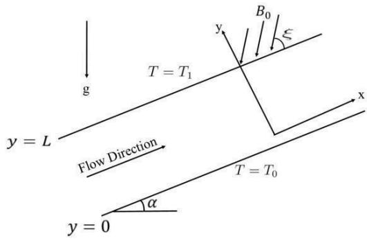
Studying in MHD Poiseuille flow has been of interest to many researchers, and more problems continue to evolve in the area of research. Several assumptions were set to control the nature of the problem to be solved in the current study. The two infinite parallel plates were inclined at an angle to the horizontal. Both plates were assumed to be non-conductors, and each was maintained at a constant temperature (the lower plate: , the upper plate ). The x-axis was positioned parallel to the parallel plates, while the y-axis was normal to the plates. An inclined magnetic field at an angle with the y-axis was applied to the parallel plates. The magnetic field developed by the fluid motion was weak and hence negligible in this study, assuming that the applied magnetic field was strong enough. Both plates were considered nonconductors to avoid the secondary component of velocity.

Fig. 1: Geometry of the problem

An electric field vector is induced whenever a fluid velocity interacts with a magnetic field . This vector is usually transverse to both V and B, as noted by Manyonge et al. [6]. Therefore;

E = V \times B\tag{0.0.1}

Let's assume that the fluid, in this case, is isotropic despite the magnetic field and use the symbol as a scalar that represents the fluid's electrical conductivity. The equation (0.0.2) below expresses the induced current's density in the fluid, designated J;

J = \sigma (V \times B)\tag{0.0.2}

Lorentz Force F is a force that co-occurs with current induced;

F = J \times B\tag{0.0.3}

Therefore, using (0.0.2) and (0.0.3);

F = \sigma (V \times B) \times B

The continuity equation is the partial differential equation expressing mass conservation. It comprises only fluid density and fluid velocity V.

\frac{\partial \rho}{\partial t} + \nabla \cdot \rho V = 0\tag{0.0.4}

The symbol represents the Gradient operator, and t stands for time. For incompressible fluid hence (o.o.4) reduces to

\frac{\partial u}{\partial x} + \frac{\partial v}{\partial y} = 0\mathrm{two-dimensional}\tag{0.0.5}

Where u, v, and w are the fluid velocity in the x, y, and z-axis directions, respectively. Maxwell's Equations express the generation and variation of electric and magnetic fields. They include;

\nabla \cdot B = 0\tag{0.0.6}

\nabla \times E = - \frac {\partial B}{\partial t}\tag{0.0.7}

\nabla \times H = J + \frac{\partial D}{\partial t}\tag{0.0.8}

Navier-Stokes Equations

The Navier-Stokes Equations for a two-dimensional steady flow are;

\rho \Big (u \frac{\partial u}{\partial x} + v \frac{\partial u}{\partial y} \Big) = F _ {x} - \frac{\partial p}{\partial x} + \mu \Big (\frac{\partial^ {2} u}{\partial x ^ {2}} + \frac{\partial^ {2 u}}{\partial y ^ {2}} \Big)\tag{0.0.9}

\rho \left(u \frac{\partial v}{\partial x} + v \frac{\partial v}{\partial y}\right) = F_{y} - \frac{\partial p}{\partial y} + \mu \left(\frac{\partial^{2} v}{\partial x^{2}} + \frac{\partial^{2} v}{\partial y^{2}}\right)\tag{0.0.10}

Where and are force components in the x and y directions, respectively, is the fluid viscosity, and p is the pressure acting on the fluid.

The force components in the Navier-Stokes equation and are mainly due to gravity. In our case, we will neglect the body forces and replace them with the Lorentz force. From equation (0.0.3), . Therefore, equations (0.0.9) and (0.0.10) becomes:

\begin{array}{r l} \rho \Big (u \frac {\partial u}{\partial x} + v \frac {\partial u}{\partial y} \Big) = & [ \sigma [ (u, 0, 0) \times B ] \times B ] \\- \frac {\partial p}{\partial x} + \mu \Big (\frac {\partial^ {2} u}{\partial x ^ {2}} + \frac {\partial^ {2} u}{\partial y ^ {2}} \Big) \\\rho \Big (u \frac {\partial v}{\partial x} + v \frac {\partial v}{\partial y} \Big) = & [ \sigma [ (0, v, 0) \times B ] \times B ] \\- \frac {\partial p}{\partial y} + \mu \Big (\frac {\partial^ {2} v}{\partial x ^ {2}} + \frac {\partial^ {2} v}{\partial y ^ {2}} \Big) \end{array}\tag{0.0.11}

respectively.

[ \sigma [ (u, 0, 0) \times B ] \times B ] = - \sigma u B _ {0} ^ {2} s i n ^ {2} \xi i\tag{0.0.13}

[ \sigma [ (0, v, 0) \times B ] \times B ] = 0\tag{0.0.14}

- \frac{\partial p}{\partial x} = \rho_{\infty} g \sin \alpha\tag{0.0.15}

Substituting (0.0.13), (0.0.14), and (0.0.15) in (0.0.11) and (0.0.12), respectively, and simplifying gives the following equations.

u \frac{\partial u}{\partial x} + v \frac{\partial u}{\partial y} = \frac{\rho_{\infty} g \sin \alpha}{\rho} - \frac{\sigma u B^{2} \sin^{2} \xi}{\rho}

+ \frac{\mu}{\rho} \left(\frac{\partial^{2} u}{\partial x^{2}} + \frac{\partial^{2} u}{\partial y^{2}}\right)

u \frac{\partial v}{\partial x} + v \frac{\partial v}{\partial y} = \frac{\mu}{\rho} \left(\frac{\partial^{2} v}{\partial x^{2}} + \frac{\partial^{2} v}{\partial y^{2}}\right)

Using the volumetric thermal expansion coefficient, be defined by;

\beta = - \frac{1}{\rho} \left(\frac{\Delta \rho}{\Delta T}\right) _ {p = c o n s t a n t} = \frac{1}{\rho} \left(\frac{\rho_ {\infty} - \rho}{T - T _ {\infty}}\right)

\rho_{\infty} = \beta\rho(T - T_{\infty})\tag{0.0.18}

Substituting (0.0.18) in (0.0.16) gives:

u \frac{\partial u}{\partial x} + v \frac{\partial u}{\partial y} = g \beta (T - T_{\infty}) \sin \alpha

- \frac{\sigma u B_{0}^{2} \sin^{2} \xi}{\rho} + \frac{\mu}{\rho} \left(\frac{\partial^{2} u}{\partial x^{2}} + \frac{\partial^{2} u}{\partial y^{2}}\right)\tag{0.0.19}

Equations (0.0.17) and (0.0.19) are the resultant Momentum Equations. The associated boundary conditions for the problem include:

u = 0, T = T_{0} \text{at} y = 0

u = 0, T = T _ {1} \mathrm{at} y = L\tag{0.0.21}

v = 0, T = T _ {0} \mathrm{at} y = 0\tag{0.0.22}

v = 0, T = T _ {1} \mathrm{at} y = L

2.1 Similarity Transformation Technique

Similarity Transformation is a technique applied in this research to convert the non-linear partial differential equations (0.0.17) and (0.0.19) into ordinary differential equations.

A two-dimensional stream function that satisfies the continuity equation is defined by and .

Let be the similarity variable, be the dimensionless temperature, and be the fluid's velocity away from the plate. Then, the following Non-dimensionless variables are used to obtain a similarity solution to the problem:

\eta = y \sqrt{\frac{U_{\infty}}{v x}}, \psi(x, y) = f(\eta) \sqrt{v U_{\infty} x}

\theta(\eta) = \frac{T - T_{\infty}}{T_{1} - T_{\infty}}

We have the following Non-dimensionless;

v \frac{\partial u}{\partial y} = \frac{U _ {\infty} ^ {2}}{2 x} (\eta f ^ {\prime} (\eta) f ^ {\prime \prime} (\eta))

\frac{\partial^{2} u}{\partial y^{2}} = U_{\infty} \sqrt{\frac{U_{\infty}}{v x}} f'''(\eta). \sqrt{\frac{U_{\infty}}{v x}} = \frac{U_{\infty}^{2}}{v x} f'''(\eta)\tag{0.0.26}

u \frac{\partial v}{\partial x} = - \frac{U_{\infty}}{4x} \sqrt{\frac{v U_{\infty}}{x}} [2\eta f'(\eta) f' (\eta) + \eta^{2} f' (\eta) f''(\eta)]

v \frac{\partial v}{\partial y} = \frac{U_{\infty}}{4x} \sqrt{\frac{v U_{\infty}}{x}} [\eta f'(\eta) f' (\eta) + \eta^{2} f' (\eta) f''(\eta)]

\frac{\partial^{2} v}{\partial y^{2}} = \frac{U_{\infty}}{2x} \sqrt{\frac{U_{\infty}}{v x}} [2f''(\eta) + \eta f'''(\eta)]

u \frac{\partial u}{\partial x} = - \frac{U_{\infty}^{2}}{2x} \eta f''(\eta) f'(\eta)

\frac{\partial^{2} u}{\partial x^{2}} = \frac{U_{\infty}}{4x^{2}} [\eta^{2} f'''(\eta) + 3\eta f''(\eta)]\tag{0.0.31}

\frac{\partial^{2} v}{\partial x^{2}} = \frac{1}{8x^{2}} \sqrt{\frac{v U_{\infty}}{x}} [8\eta f'(\eta) + 7\eta^{2} f''(\eta) + \eta^{3} f'''(\eta)]

\text{Let} = \frac{g\beta(T_{1}-T_{\infty})x}{U_{\infty}^{2}}, Re = \frac{U_{\infty} x}{\nu} \text{and} M = \frac{x\sigma B_{0}^{2}}{U_{\infty}\rho}

Substituting (0.0.24), (0.0.25), (0.0.26), (0.0.30), (0.0.31), (0.0.33) and in (0.0.19) gives;

4\theta Gr \sin \sin \alpha - 4M \sin^2 \xi f' + \frac{1}{Re} \left[ \eta^2 f''' + 3\eta f'' \right] + 4f''' = 0

Substituting (0.0.27), (0.0.28), (0.0.29), (0.0.32), (0.0.33) and v = in (0.0.17) gives;

\sqrt {R e} [ - 2 \eta f ^ {\prime} f ^ {\prime} - 8 f ^ {\prime \prime} - 4 \eta f ^ {\prime \prime \prime} ]

- \sqrt {\frac {1}{R e}} [ 8 \eta f ^ {\prime} + 7 \eta^ {2} f ^ {\prime \prime} + \eta^ {3} f ^ {\prime \prime \prime} = 0\tag{0.0.35}

Equating equation to equation and collecting the like terms together gives;

4\theta Gr \sin \alpha + \left[ 2\sqrt{Re}\eta f' + 8\sqrt{\frac{1}{Re}}\eta - 4M \sin^2 \xi \right]f'

\left[ + \frac{3\eta}{Re} + 8\sqrt{Re} + 7\sqrt{\frac{1}{Re}} \eta^{2} \right] f^{’’} +

\left[ 4 + 4 \sqrt{Re} \eta + \sqrt{\frac{1}{Re}} \eta^{3} + \frac{\eta^{2}}{Re} \right] f^{\prime \prime \prime} = 0\tag{0.0.36}

Equation (0.0.36) is the momentum equation to be solved with boundary conditions; with boundary conditions;

f = 0, f ^ {\prime} = 0, \theta = 1 \mathrm{at} \eta = 0

f ^ {\prime} = 1, \theta = 0 \mathrm{at} \eta = \infty\tag{0.0.37}

2.2 Shooting Method

The non-linear ordinary differential equations (0.0.36) with boundary conditions (0.0.37) were solved numerically using the shooting method.

III. RESULTS AND DISCUSSION

The nonlinear equations with boundary conditions were solved numerically using the shooting method. The boundary value ODEs were converted using the shooting method technique utilizing Secant iteration into a group of first-order initial values for ODEs. The fourth-order Runge-Kutta technique, incorporated within Mathematica software, was then used to solve the resulting system. In figures (fig. 2 - 6), velocity distributions were displayed for various governing parameters to analyze the results of the numerical calculations. Physically realistic numerical values were assigned to the embedded parameters in the system to obtain an insight into the flow structure for velocity.

Figure 2 shows that parallel plates' inclination angle to the horizontal impacts fluid velocity. There is a rise in fluid velocity whenever the parallel plates' angle of inclination, , increases. The impact of the magnetic field's inclination angle ( ) was also determined. According to Figure 3, increasing decreases the fluid velocity. Figure 4 shows that there is an influence of on fluid velocity. A rise in fluid velocity is expected whenever value increases. Another parameter that affects fluid velocity is the Hartmann number, M. Increasing the Hartmann number increases the fluid's velocity, as shown in Figure 5. Lastly, a Reynolds number's influence on fluid velocity was noted. A rise in its values results in a drop in the fluid velocity, as shown in Figure 6.

{"image_source":{"path":"images/a514ebc4593b49d81d65f521311f205d06ba97f2a59ed96221ed657a62334421.jpg"},"content":"","chart_caption":[{"type":"text","content":"Fig. 2: Velocity at different "},{"type":"equation_inline","content":"\alpha"}],"chart_footnote":[]} {"image_source":{"path":"images/d212dccb10d006b85001373be11607959ebefd3f633248e40df474bca535ac3a.jpg"},"content":"","chart_caption":[{"type":"text","content":"Fig. 3: Velocity at different Gr"}],"chart_footnote":[]}

{"image_source":{"path":"images/7b1886b40212336824c35e6cf7849f123461a2ce53c7e3ce9c9b01297e0d8238.jpg"},"content":"","chart_caption":[{"type":"text","content":"Fig. 4: Velocity at different M"}],"chart_footnote":[]} {"image_source":{"path":"images/95a79dac86381baa615eedb4eb5753c68f77b2a3034ecc4ccf9c34965acc5a8f.jpg"},"content":"","chart_caption":[{"type":"text","content":"Fig. 5: Velocity at different Re"}],"chart_footnote":[]}

{"image_source":{"path":"images/36996f8f7ea8c504044f2fce9e64a878674dd40cb42a57594604d54dc1736d44.jpg"},"content":"","chart_caption":[{"type":"text","content":"Fig. 6: Velocity at different "},{"type":"equation_inline","content":"\xi"}],"chart_footnote":[]}

IV. CONCLUSION

This paper examined two-dimensional steady MHD free convective Poiseuille flow past an inclined magnetic field and two infinitely inclined parallel plates. The impact of inclining the magnetic field and parallel plates and other pertinent parameters on the velocity and temperature of the fluid were discussed. Differential governing equations were formulated and solved using numerical methods. According to the results, a rise in the parallel plates' inclination angle to the horizontal, Grashof number, and Hartmann number raises the fluid velocity. Besides, increasing the magnetic field's inclination angle and the Reynolds number drops the fluid velocity. The research findings are applicable in the manufacturing industry, electrical equipment cooling, nuclear reactor insulation, and crystal growth in liquids.

− Conflict of Interest

The authors declare no conflict of interest.

− Ethical Approval

Not applicable

− Data Availability

The datasets used in this study are openly available at [repository link] and the source code is available on GitHub at [GitHub link].

− Funding

This work did not receive any external funding.

− References

8 Cites in Article

REFERENCE FORMAT

− Cite this article

Generating citation...

Classification
1

LCC Code:QC521-526
Version of record

v1.0
Issue date

06 May 2024
Language

en

Research scientists analyzing DNA structures in a digital environment.

Download Article

Open Access

Research Article

CC-BY-NC 4.0

Views 501

Downloads 19

Year

Special Issue

Launch a focused special issue to highlight research, emerging trends, and expert insights in your academic field.

Keywords

5

Free convective Inclination MHD Poiseuille flow Runge-Kutta method.

The Effect of Plate and Magnetic Field’s Inclination on Fluid Velocity of an MHD Free Convective Poiseuille Flow

IntelliPaper

− Abstract

− Explore Digital Article Text

I. INTRODUCTION

II. NUMERICAL SOLUTION OF AN ORDINARY DIFFERENTIAL EQUATION

2.1 Similarity Transformation Technique

2.2 Shooting Method

III. RESULTS AND DISCUSSION

IV. CONCLUSION

− Conflict of Interest

− Ethical Approval

− Data Availability

− Funding

− References

− Cite this article

Classification

Version of record

Issue date

Language

Special Issue

Keywords

Next Research

Copy of Cardiovascular Risk Factors and Cardiovascular Risk in People Living with HIV: Comparison of Four Cardiovascular Risk Prediction Algorithms

Privacy preferences

The Effect of Plate and Magnetic Field’s Inclination on Fluid Velocity of an MHD Free Convective Poiseuille Flow

IntelliPaper

Request Review Access

Order Article Reprints

− Abstract

− Explore Digital Article Text

I. INTRODUCTION

II. NUMERICAL SOLUTION OF AN ORDINARY DIFFERENTIAL EQUATION

2.1 Similarity Transformation Technique

2.2 Shooting Method

III. RESULTS AND DISCUSSION

IV. CONCLUSION

− Conflict of Interest

− Ethical Approval

− Data Availability

− Funding

− References

− Cite this article

− Related Research

Classification

Version of record

Issue date

Language

Special Issue

Keywords

Next Research

Copy of Cardiovascular Risk Factors and Cardiovascular Risk in People Living with HIV: Comparison of Four Cardiovascular Risk Prediction Algorithms

Privacy preferences