




IntelliPaper
Abstract
The present investigation was based on analyzingthe signal generated by the electromagnetic spectrum displayequipmentSAG4400L-NWT4000. Taking in to accountan operating range of 850-1900 MHz of a mobile operator. With the use of this device, it was possible to compare the the or eticalvs. experimental postulates obtained through the tests carriedoutinthisstudy.
Explore Digital Article Text
I. INTRODUCTION
Radio communication is defined as telecommunication by means of radio waves, which are electromagnetic waves propagating without artificial guidance at frequencies below 3,000 GHz. Technically radiation is an outgoing flow of electromagnetic energy from any source, while emission is the radiation by a transmitting station [1].
The birth of GSM (Groupe Special Mobile) technology took place in Europe in 1982, within the framework of the European Conference of Postal and Telecommunications Administrations, with the aim of bringing together the digital and mobile communication systems existing at the time. [1]. The possibility of design allowed several operators to share the spectrum, so that users can connect to their preferred network. Consequently, signals can be seen as a function of frequency, through a spectrum analyzer. Using the SAG4400L-NWT4000-35MHz-4.4GHz device, it is possible to determine the electromagnetic spectrum traffic in the 850-1900MHz frequency of an operator. In addition, the formulas involving the analysis of electromagnetic waves are presented in a theoretical way.
II. SAG4400L SPECTRUM ANALYZER
The SAG4400L spectrum analyzer can measure the frequency bands from 35MHz to 4.4GHz. The functions of the device are described below. [2]
2.1 Specifications
Table 1: Sag4400l Spectrum Analyzer Technical Specifications
| Input-output frequency range | 35 MHz – 4,4 GHz |
| Input-output frequency measurement | 1kHz |
| Maximum Input Power | +8dBm |
| Noise Level | -70 dBm |
| Intermediate Frequency Bandwidth (IF) | 250 kHz*2 |
| Measurements | 120*65*25 |
| Source | +5v/0,35 A |
The SAG4400L electronic device consists of two plugs. An input (IN) for the signals to be analyzed. In turn, an output (OUT), which generates the spectra corresponding to certain values.
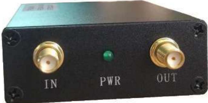 Fig. 1: External View of SAG 4400L-NWT4000 Device
The interior is composed of two sections: The signal generator and spectrum analyzer. It means that both parts are connected, through a Serial to USB converter, allowing the installation of the corresponding software for simulation.
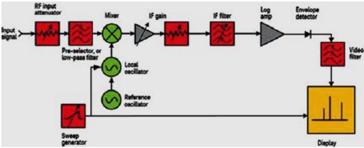 Fig. 2: Block Diagram of a Superheterodyne Spectrum Analyzer
In general, the blocks that make up the SAG4400L-NWT4000 Spectrum Analyzer are analyzed. In the first instance, the signal capture uses a connector on the input signal. In turn, it enters through a high-pass filter block to avoid the high frequencies of 4.4GHz. Next, there is the schematic of a multiplexer that combines the incoming signal with one emitted from the ADF4350 generator, at a frequency of 1 GHz. [3]. In the next block, there is a low-pass filter to eliminate frequencies lower than those set by the software. On the other hand, the diagram of a logarithmic signal amplifier is shown. Finally, the logarithmic signal arrives to an ATMEGA microprocessor that is in charge of capturing the samples and sending them to the software, by means of the RS-232 to USB converter (FT232).
2.3 WinNWT4 Software Configuration
The WinNWT4 software allows to visualize spectra, generate signals, by means of an interactive configuration panel. Consequently, the availability of measuring the power of a signal is feasible.
When installing the program, the USB port of the computer must be configured to recognize the SAG440L-NWT4000 device. If the installation fails, the drivers distributed by the device manufacturer must be installed. It is essential to indicate the serial port that the computer has in order to be compatible with the program.
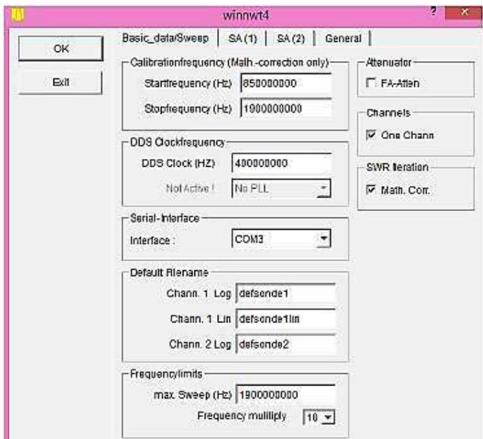 Fig. 3: WinNWT4 configuration window
2.4 SAG4400L Device Configuration
Once the port number is identified, the program is run to configure the spectrum analyzer function. In the main window of the software, go to the (Setting's) tab and choose the (Options) display; a tab is generated according to Fig.4. Then select the Serial-USB port number in the (Serial-interface) option, this port must match the found device manager port. Now, set the frequency ranges for the band to be analyzed. To do this, go to the option (Calibration Frequency), where the start frequency of the band is set to (Start frequency) and the end frequency to (Stop frequency). The item (DDS Clock frequency) is the frequency at which the device will be sampled. The recommendation is to set it to 1 GHz. For the (Frequency limits) tab, enter the Maximum Sweep Frequency and modify the Adjustment Rate for the signal. By default, the real frequency is assumed as a multiplication factor of the display frequency * 10.
Now, enter the main program window and in the (Mode) block, select (Sweep mode), only to analyze spectra. Finally, the delay time (Interrupt's) is set, which is used to assume the delay time in the capture of the measurements, through the power of each sample. The recommendation is to leave the value fixed at: 0 s.
III. CONCEPTOS FUNDAMENTALES
3.1 Magnetic Field
A magnetic field is a region of space where magnetic forces exist, forces that attract or repel metals. It is an invisible field that exerts a magnetic force on substances that are sensitive to magnetism. [4] [5].
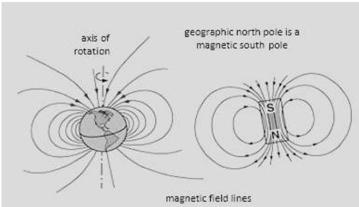 Fig. 4: Interpretation of the Magnetic Field
Magnetic field lines are a way of representing this magnetic field. Magnetic fields can be generated by magnets or by electric currents. The lines tell us how strong the field is and how far its action reaches. [6]
3.2 Electric Field
The electric field is the region of space in which the electric force interacts, or a physical field that is represented by a model describing the interaction between bodies and systems with properties of an electrical nature.
3.3 Electric Field Strength
A The electric field strength (E) at a point is a vector quantity representing the electric force (F) acting per unit of positive witness charge, which located at that point is mathematically defined as:
3.4 Power
Electrical power is a parameter that indicates the amount of electrical energy transferred from a generating source to a consuming element per unit of time.
3.5 Bandwidth
In Internet connections, bandwidth is the amount of information or data that can be sent over a network connection in a period of time. [6]
3.6 Maxwell's Equations
These equations are considered the basis of all electrical and magnetic phenomena
Gouss Low
Gauss Low of Magnetism
Foraday Law
Ampere-Maxwell Low
Fig. 5: Maxwell's Equations
3.7 Electromagnetic Waves
An electromagnetic wave is composed of an electric field and a magnetic field as a function of time, electromagnetic waves carry power and this can be determined through the Poityng Vector which determines the power flux density. The formula is defined as follows
3.8 Sinusoidal Electromagnetic Waves
They are waves that travel at the speed of light, and the magnetic and electric fields are perpendicular to each other; these waves obey the principle of superposition.
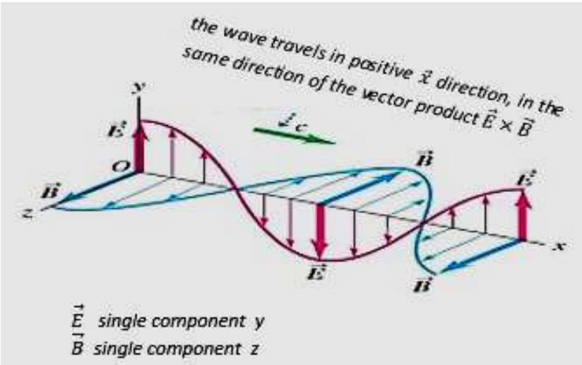 Fig. 6: Sinusoidal Electromagnetic Wave Polarized Through the X-Axis
3.9 Wavelength
When an electromagnetic wave is analyzed in a small part of vision can be made relation of this as if it were a plane wave. The frequency f, the wavelength and the speed of propagation c have a close relationship therefore:
IV. ANALYSIS PARAMETERS (CALCULATIONS)
According to the regulations of the International Commission on Non-Ionizing Radiation Protection (ICNIRP). It establishes parameters for the Electric Field Intensity and Magnetic Field Intensity allowed in a population profile. These values allow the development of Theoretical Calculations.[8] For a frequency range between 400-2000MHz the equations for Electric Field Strength, Magnetic Field Strength and Plane Wave Power Density (Poityng) are, given in (V/m), (A/m), (W/m ):
4.1 Sample 1 of 850-950 MHz
Data:
(vacuum permeability)
(medium permittivity)
(speed of light)
a) Average Frequency
b) Wavelength
c) Electric Field Strength
d) Magnetic Field Strength
e) Power Density
f) dBm power
The calculations are carried out in the same way for each of the frequencies involved in the analysis.
The operator has GSM technology; 2G-3G network for frequencies between 850-1900 MHz and for 4LTE technology 4G network frequencies between 1700-2100 MH.
Table 2: Frequency Band -Mobile Operator
| Technology | Frequency | Network | Service |
| GSM | 850 /1900 MHz | 2G-3G | Voice and Data |
| 4LTE band | 1700/ 2100 MHz | 4G | Data |
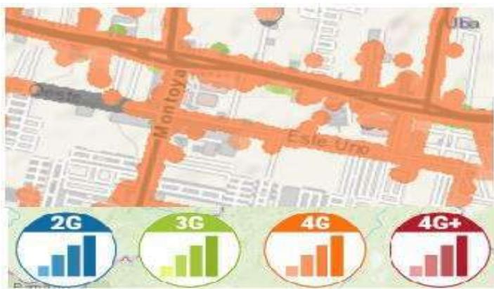 Fig. 7: Operator Coverage Area
5.1 2G and 3G network
These are networks that can be connected to a cellular phone when a user is in remote locations, such as rural or mountainous areas. With 2G networks the speed is lower and generally voice has preference over data, and these two services cannot work at the same time.
The main difference between 3G and 2G networks is that 3G offers faster browsing speeds; moreover, with 3G networks on a phone or tablet, voice and data services can operate at the same time.
5.2 4G Network
They represent the fourth generation of mobile telephony technologies. These networks represent the next step up from the current 3G and are available to customers. With them, the data network improves in quality and speed, allowing speeds of up to 75 Mbps downstream (download) and 25 Mbps upstream.
VI. RADIO FREQUENCY SPECTRUM ANALYSIS
Spectrum analyzer allows plotting the amplitudes or levels of the frequencies of a specific signal. The 35MHz-4.4GHz SAG4400L-NTW4000 device has been used. This device will be used to determine the electromagnetic spectrum traffic in the 850-1900MHz frequency of the operator in the area determined for measurements. In turn, 6 samples have been taken in the above-described range for their respective comparison.
Table 3: Device Configuration Parameters Sag4400l-Nwt4000, Frequency Range 890-1900 Mhz
| Starfrequency (Hz) | 850000000 Hz | Initial Frequency |
| Stop Frequency (Hz) | 1900000000 Hz | Frequency Final |
| DDSclock (Hz) | 40000000 MHz | Sampling Synchronization |
| Frequency limits (Hz) | 1900000000 Hz | Spectrum Sweep Frequency |
| Frequency multiple | 10 | Multiplication Factor for Plotting the Signal |
| Average Power (dBm) | -74,425 |
{"image_source":{"path":"images/bc0995d5cc64d3827f0a0ccd221e8cc98905f3ccfd9402319be64a53d87b5dc5.jpg"},"content":"","chart_caption":[{"type":"text","content":"Fig. 8: Frequency Spectrum Plot of the Operator's Band. With the SAG4400L-NWT4000 Spectrum Analyzer Equipment Between 850-1900 MHz"}],"chart_footnote":[]}
Interpreting the graph in Fig. 8. The decibels (dBm) of incidence of the weighting is observed in the 800-1500 MHz band, note that the maximum peaks of before and after due to the data traffic located approximately in the 1700MHz.
Then, 6 samples have been selected, divided between the 850-1450 MHz range {"image_source":{"path":"images/250707c6a1a6395aaa6b277e7cfc45f2809b1cbed00776cc7e082ab2fb23cce7.jpg"},"content":"","chart_caption":[{"type":"text","content":"Fig. 9: Sample 1: Plot of the Frequency Spectrum of the Band. With the Spectrum Analyzer SAG4400L-NWT4000 Between 850-950MHz"}],"chart_footnote":[]}
{"image_source":{"path":"images/b7214fed76d6a0ff72058a470e39d3010d243a4910fc4b758b3b44641e9e7601.jpg"},"content":"","chart_caption":[],"chart_footnote":[]} {"image_source":{"path":"images/a9afa2400e3b281336cfbbd79f0c3e6867445274c85601fdc183228a7ab2d4c7.jpg"},"content":"","chart_caption":[{"type":"text","content":"Fig. 10: Sample 2: Plot of the Frequency Spectrum of the 950-1050 MHz Band with the SAG4400L-NWT4000 Spectrum Analyzer"}],"chart_footnote":[]}
{"image_source":{"path":"images/10f4b9a669a370409a9ad75c91ca5dfcdbb0aa281c6409ea4aa9f545b9124dc3.jpg"},"content":"","chart_caption":[{"type":"text","content":"Fig. 11. Sample 3: Plot of the Frequency Spectrum of the Band. With the Spectrum Analyzer SAG4400L-NWT4000 Between 1050-1150 MHZ"},{"type":"text","content":"Fig. 12: Sample 4: Plot of the Frequency Spectrum of the Band. With the Spectrum Analyzer SAG4400L-NWT4000 Between 1150-1250 MHz"}],"chart_footnote":[]} {"image_source":{"path":"images/85b64f3d2ead3e9a7e5769da60ba89d72b69af6dd42da4dc17213280369eaa54.jpg"},"content":"","chart_caption":[],"chart_footnote":[]}
{"image_source":{"path":"images/387d286e280017787563dde293fc2f14c8ab979ee5bed37fa324d3f77477f064.jpg"},"content":"","chart_caption":[{"type":"text","content":"Fig. 13. Sample 5: Plot of the Frequency Spectrum of the Band. With the SAG4400L-NWT4000 Spectrum Analyzer Equipment Between 1250-1350MHz"},{"type":"text","content":"Fig. 14. Sample 6: Plot of the Frequency Spectrum of the Band. With the Spectrum Analyzer SAG4400L-NWT4000 Between 1350-1450 MHz"}],"chart_footnote":[]}
Table 4: Experimental Comparative Power Analysis of the Sag4400l-Nwt4000 Operator Frequencies, Frequency Range 890-1550 Mhz
| Rango de Frecuencias (MHz) | Potencia Máxima (dBm) | Potencia Mínima (dBm) | Potencia Promedio (dBm) | Potencia Calculada (dBm) |
| 850 - 950 | -69,36 | -86,18 | -77,77 | -76,15 |
| 950 - 1050 | -69,65 | -85,99 | -77,82 | -76,37 |
| 1050 - 1150 | -65,15 | -85,61 | -75,38 | -76,58 |
| 1150 - 1250 | -69,65 | -86,37 | -78,01 | -78,77 |
| 1250 - 1350 | -79,11 | -85,99 | -82,55 | -81,95 |
| 1350 - 1450 | -65,15 | -86,57 | -75,86 | -77.11 |
VII. CONCLUSIONS
The SAG4400L device generates Radio Frequency waves, these were validated and the data obtained were compared with the theoretical values for such frequencies, by simulating the mathematical models used by the laws of electromagnetism. On the other hand, it is evident that the transmission power in the frequency range between 850-1950 MHz is within the levels established by the International Telecommunication Union (ITU) Standards. Consequently, the theoretical and experimental power values, measured in dBm, are similar. Finally, by generating more data traffic in the different frequency categories analyzed, more peaks, disturbances or disturbances (noise) are generated when visualizing the graph of such measurements.
Conflict of Interest
The authors declare no conflict of interest.
Ethical Approval
Not applicable
Data Availability
The datasets used in this study are openly available at [repository link] and the source code is available on GitHub at [GitHub link].
Funding
This work did not receive any external funding.
References
Cite this article
Related Research



Special Issue
Launch a focused special issue to highlight research, emerging trends, and expert insights in your academic field.
