Reliability of the Bond Graph Approach for Robust Diagnosis of a Newborn Incubator System

Dr. Sellami Abderrahmene

IntelliPaper

Peer Review Double Blind Handling Editor
Accepted 1 January 2024 Access Review Comments
Online published 17 January 2024

− Abstract

This article aims to solve a problem of research with a thermal system (incubator) to the graph of pseudo-connections. The method we develop is based on the determination of the resolution on the model ARR-BGM (Analytical Redundant Relationships Bond Graph). These relationships serve to detect and isolate faults in the various elements of the system, but also to locate the industrial system. We introduced defects in the heat source, leaks in the incubators and a leak in the incubator door; these defects were transferred by thermal transfer to negative values. The results of simulation, the effectiveness of proposed method to detect and locate defects, in addition, to analyze the robustness of the Incubator to defects, we imported the graphical link model as linear fractional transformations (BG-LFT). This makes it possible to verify the reliability of the approach of the link graphs in terms of sensitivity and detectability of defects that may appear in an industrial system.

− Explore Digital Article Text

I. INTRODUCTION

The main objective of the automation engineer is to determine control algorithms of physical systems that are often of different natures, electrical, mechanical, hydraulic, thermal, etc. This objective will not be obtained if the system modeling is not validated which is the first task. The model describing physical reality is usually obtained on the basis of an idealized description of the system and only dominant phenomena are often taken into account given the complexity and diversification of the system .

In this article we chose the incubator not only for the complexity of the system but also the importance of this system in the lives of human beings. An incubator is a protected heated place, which allows the development and monitoring of certain newborns. It is an apparatus intended to allow the normal development of children born before term (premature), or fragile newborns .

The incubators consist of an electrical part (electrical heating resistance) and a thermal part (enclosure receiving the child). Several elements of the incubator can be a source of contamination of the environment of the newborn. Indeed, each part constituting the incubator has specificities for cleaning, disinfection and maintenance. In addition, disinfection is a priority of neonatology units [11], but maintenance (sealing problem, problem of thermal insufficiency or overheating) is a task for technicians [12-15]. To facilitate the task of the technicians, it is necessary to find a reliable and generous approach to model and analyze the defects that may appear during operation this incubator. This reliability and generosity can be found in several approaches such as Petri nets [16-24] and bond graph [25-30].

Most authors have limited their research to a mathematical model to simulate the different heat exchanges in the incubator or for control purposes.: Ultman [31] developed a simulator of neonatal energy transfer to provide a convenient yet precise comparison of sensible heat loss in incubators, Le BIanc [32] described the fundamental equations involved in thermal exchange between infants and their environment. Simon [33] developed a Theoretical Model of Infant Incubator Dynamics. Pauline Décima[34] developed a Mathematical modeling of thermoregulation processes for premature infants in closed convectively heated incubators and for calculating thermo neutrality in closed incubators for premature newborns, Zermani [35] developed a simulation model of infant-incubator system with decoupling predictive controller, Andrés Fraguela [36] Proposed a model of heat exchange and energy balance in premature newborns during the first hours of life in a closed incubator. In addition, a control problem was proposed and solved in order to maintain thermal stability of premature. Stéphane Delanaud [37] proposed a New Software for assessing the impact of humidity on the optimal incubator air temperature.

The bond graph approach is a very effective approach for this kind of system, since it is multidisciplinary and was initially used for modeling physical systems. The usual approach of the users of this approach is to consider the bond graph model as a knowledge model for the simulation of dynamic systems. The idea of using a single representation (the bond graph) for the modeling, analysis and synthesis of control laws by exploiting causality has been developed in this field .

Engr Hassan Javed and Asif Mahmood Mughal [41] have developed a flow chart model for an incubator that only takes into account the heating part modeled as heating capacity, then the heat flux in the chamber is modeled as a flux source, but they neglected the thermal capacity of the external environment and the thermal capacity of the mattress. In this paper we propose a new approach of modeling by the bond graph approach of the incubator taking into account the thermal capacities of the environment as well as the mattress.

The purpose of this article is also to design a robust diagnostic system based on a model using a single tool: the link graph. Methodologically, the work consists of automating model generation and failure indicator procedures in the form of fractional linear transformations (LFTs) and interchangeably for integration into the supervisory system. At the industrial level, the results obtained were applied to real installations: incubator.

II. MATHEMATICAL MODEL OF THE INCUBATOR

The incubator can be described as a reaction system consisting of two large dynamic parts: the climate inside the lodge and the heating system. The heat, humidity and oxygen at the thermostat outlet are defined as input variables of the incubator and the climate parameters tested by the newborn are the output variables. The temperature of the box, the temperature of the walls and the windows intended for medical care, the incubator consists of three main parts:

The ambient air in the lodge
The mattress;
The walls.

2.1 Modeling the Thermostat

To model this part of the incubator, consider the following simplifying measures:

The thermostat is assumed to be homogeneous with constant characteristics such as specific heat
The temperature distribution is uniform,
The specific heat is equal to that of the normal air.

The temperature of the air coming from the thermostat can be written as follows:

\frac{d T _ {h a}}{d t} = \frac{(T _ {h a i} - T _ {h a})}{C . R _ {p m}}\tag{1}

2.2 The Ambient Air in the Lodge

The ambient air of the incubator box exchanges heat with all the elements of the Child-incubator system mainly by convection, but also by mass transfer during the Breathing and also by evaporation. In our case we consider the incubator without baby. During a period dt, the thermal equilibrium of the ambient air of the box can be determined according to the following equation:

\frac{d T _ {a}}{d t} = \frac{Q _ {h t} - Q _ {a c v} - Q _ {m a t}}{M _ {a} . C _ {p a}} ag{2}

Where denotes the air mass in the box and its thermal capacity.

The ambient air of the box gives heat to the walls of the incubator by convection. This energy is determined by the following equation:

Q_{acv} = h_{acv}.A_{w}.(T_{a} - T_{w})\tag{3}

Where is the surface of the walls in contact with the air. The convective transfer coefficient depends mainly on the shape of the incubator, the ventilation in the box and the number of Nusselt and Reynold.

The mattress surface of the incubator not occupied by the child also exchanges the energy with the convective ambient air according to the following equation:

Q_{mat} = h_{acv}. A_{net}. (T_{a} - T_{m})\tag{4}

Where is the surface of the mattress in contact with the air.

2.3 Thermal Balance of the Walls

The walls of the incubator, made of transparent Plexiglas, have six portholes and a window provided for care. The walls consist of a single homogeneous layer thw thickness equal to 6mm and the heat distribution is uniform on the inner surface and external.

The thermal equilibrium during a time dt can be written in the following way:

\frac{d T _ {w}}{d t} = \frac{Q _ {a c v} - Q _ {c v 0} - Q _ {r 0}}{M _ {w} . C _ {p w}}\tag{5}

Where Mw the total mass of plexiglass walls and its thermal capacity.

The inner surface of the incubator wall receives convective heat loss from the ambient air in the incubator Qacv.

On the other hand, the walls of the incubator exchange with the neonatology room of radiation and convection energy. The convective heat transfer is determined by the equation below:

Q_{cv0} = h_{cv0}.A_{wt}.(T_{w} - T_{e})\tag{6}

The heat transfer by radiation is calculated by the following relation:

Q_{r0} = A_{wt}.\delta.\xi_w [(T_w + 273.15)^4 - (T_e + 273.15)^4]

2.4 Mattress Modeling

The mattress of the incubator exchanges heat by conduction of the ambient air and skin conduction. In the case of an empty incubator the thermal equilibrium of the mattress can then be written in the same way next:

\frac{dT_{m}}{dt} = \frac{Q_{mat} - Q_{ic}}{M_{m}.C_{pm}}\tag{8}

Knowing that the two plates of the support that carries the mattress are thin, and the surface of small contact, the transfer of heat by conduction of the mattress to the incubator, , is not considerable and can be ignored.

III. INDUSTRIAL SYSTEM BY BOND GRAPH MODELS

The bond graph formality was introduced by H. Paynter in 1961 [42] and formalized by Karnopp and Rosenberg in 1975 [43]. The bond graph tool is now used regularly in a few companies, particularly in the automotive industry (PSA, Renault, Ford, Toyota, General Motors, etc.). This method illustrates energy transfers in the system using power bonds. A power link is symbolized by a half arrow, whose orientation indicates the direction of power transfer. Thus, figure 1 shows the power transfer from subsystem to subsystem [44-46]. One of the fundamental characteristics of the bond graph formalism is its unifying aspect, whatever the physical domain of application (electrical, mechanical, hydraulic, chemical...). We can visualize energy transfers in multi-domain systems using the generalized variables presented in the next section. The notion of power is described by the following relation:

\[P(t) = e(t).f(t)\]

This equation illustrates energy transfers in the system by using power bonds. A power link is symbolized by a half arrow, whose orientation indicates the direction of power transfer. Thus, figure 1 shows the power transfer from subsystem to subsystem .

Each power link carries two information's simultaneously: the effort and the flow (see figure 1). These are the generalized power variables (their product being the transferred power).

Figure 1: Power link

IV. ROBUST DIAGNOSIS OF INDUSTRIAL SYSTEM BY BOND GRAPH MODELS

Linear Fractional transformations (LFT) are generic objects widely used in the modeling of uncertain systems. The universality of fractional linear transformations is reached seen that any rational expression can be written in this form . This form of representation is very used for the synthesis of control laws of uncertain systems using the principle of -analysis. It consists of separating the nominal part of a model from its uncertain part, as shown in figure 2.

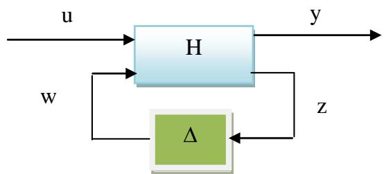Figure 2: Representation of the Fractional Linear Transformations (LFT)

The nominal values are grouped together in an augmented matrix denoted H, supposed to be proper. The uncertainties whatever their types (structured and unstructured parametric uncertainties, modeling uncertainties, measurement noises, etc.) are combined in a matrix of diagonal structure.

With:

: System state vector;

: Vector grouping system control inputs; : Vector grouping the measured outputs of the system;

and : Respectively include inputs and auxiliary outputs. n, m, l and p are positive integers.

4.1. Construction of a BG-LFT Model

All industrial systems can be modeled by BG model according to figure 3. Indeed, the input signal is modeled by an effort source (Se) or a flow source (Sf). The complete system is modeled by resistive elements (R) and storage elements (I or C), while the detectors are modeled by detector elements (De or Df).

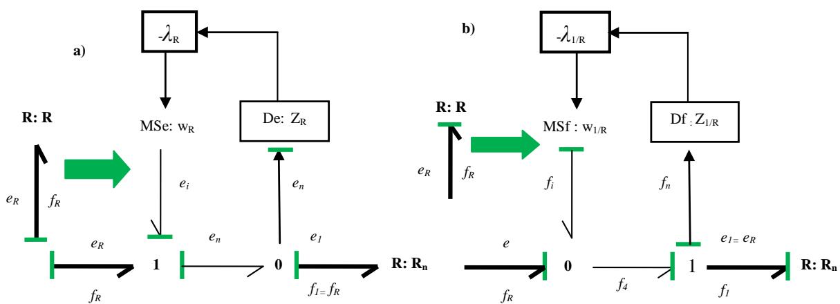Figure 4: a) BG-LFT Model of an Element Resistance with Multiplicative Uncertainty, b) BG-LFT Model of an Element Conductance with Multiplicative Uncertainty

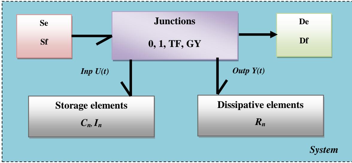Figure 3: Industrial System Described by Bond Graphs 4.2. Bond Graph Element With Multiplicative Uncertainty

The introduction of a multiplicative uncertainty on e.g. element R in causality gives resistance:

e_{R}=R_{n}(1+\lambda_{R})f_{R}=e_{n}+\lambda_{R}e_{n}=e_{n}+e_{inc}\tag{10}

With:

: The nominal value of the element ;
: The multiplicative uncertainty parameter;
et : Represent respectively the effort and the flow in the element ;
et : Respectively represent the effort made by the nominal setting and effort introduced by the additive uncertainty.

Unlike the force introduced by an additive uncertainty with respect to the parameter (equation (1)), the force provided by a multiplicative uncertainty (equation (10)) is a function of the force provided by the nominal parameter. This is an important property for the parametric identification step and the supervision step.

4.3 Resistive Element With a Multiplicative Uncertainty

The bond graph model equivalent mathematical model of equation (2) is given in figure 4.

4.4 Storage Elements With a Multiplicative Uncertainty

Parts C derived causality

The bond graph model equivalent mathematical model of equation (2) is given in figure 5.

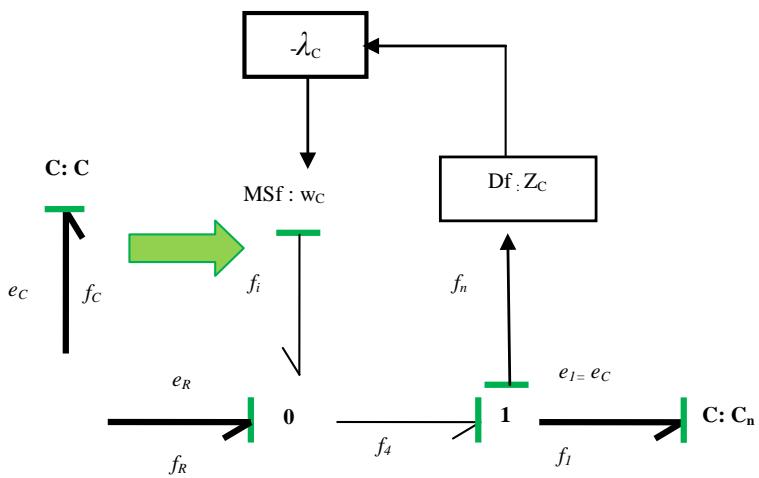Figure 5: BG-LFT Model of an Element C in Derivative Causality With Uncertainty

• Parts C Integral Causality

The bond graph model equivalent mathematical model of equation (2) is given in figure 6.

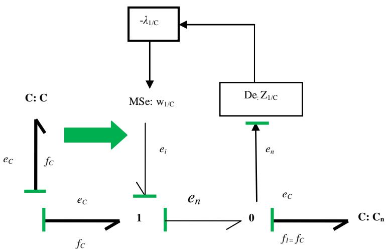Figure 6: a) BG-LFT Model of an Element C in Integral Causality with Multiplicative Uncertainty

To determine the final model that fits the model of a physical system by the Bond Graph approach and the Linear Fractional transformations model, we must integrate according to the following figure 7.

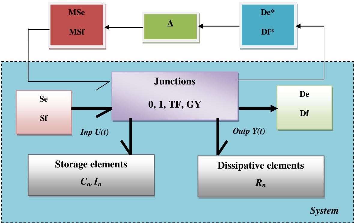Figure 7: BG-LFT Model for Physical System

4.5 Generation of Robust Residuals

To determine the residuals by the redundant analytical relationship (ARR), the following steps must be followed:

phase: Determining the derivative model;
phase: Determining the graph model using the LFT transform;
phase: Determining the residual equations for the two junctions (o and 1).

For a o-junction:

\sum f _ {\text { inc }} + \sum S f + \sum w _ {i}\tag{11}

For a 1-junction:

\sum e_{inc} + \sum Se + \sum w_{i}\tag{12}

With, and are unknown variables. Moreover, the sum of flow sources and the sum of the effort sources are respectively performed at the level of the o-junction and the 1-junction.

then determine the residue equations at their junctions.

ARRS : \Phi(\dot{\sum} Se, \sum Sf, De, Df, \sum w_{i}, R_{n}, I_{n}, C_{n}, TF_{n}, GY_{n})

where

and are nominal elements TF and GY. , and are nominal elements R, C and I.

are uncertainties on the junction-related items.

V. ANALYSIS OF RESIDUALS SENSITIVITY

The methods of analysis of sensitivity to uncertainties and defects is proposed to improve diagnostic performance has been developed in recent years . Indeed, these methods are unfortunately not effective for the generation of residues since they neglect the inter-parametric correlation (the thresholds are often overvalued and may differ). In addition, the Bond Graph tool provides an effective solution to the problem of parametric dependencies since the generation of bond graph using (BG-LFT) automatically separates the residuals and the adaptive thresholds, this separation clearly showing the energy contribution of the uncertainties to the indicators of defects and facilitating their assessments in the decision stage by calculating the adaptive thresholds of normal operation. The diagnostic performance is controlled by an analysis of the sensitivity of the residues to uncertainties and defects. To improve diagnostic performance, determine the indices performance (sensitivity index and detectability index) .

5.1 Sensitivity Index (SI)

The index of parametric standardized sensitivity explained the evaluation of the energy provided by the residue uncertainty on each parameter by comparing it with the total energy provided by all uncertainties.

SI_{n} = \frac{\left| w_{i} \right|}{d_{n}}\tag{14}

: Uncertainty on the parameters
: Basic element bond graph model and )
: Modulated entry for Uncertainty in the parameters

5.2 Detectability Index (DI)

The detectability index represents the difference between the efforts (or streams) provided by defects in absolute terms and that granted by all the uncertainties in absolute value.

Junction 1
Junction o

DI = \left| Y_{i} \right\| f_{in} \bigg | + \left| Y_{s} \right| d\tag{16}

While defects detectability conditions will be:

The defect is not detectable:
The defect is detectable:

VI. MODELING AND SIMULATION RESULTS OF INCUBATOR BY BOND GRAPH MODELS

6.1 Incubator System

In this subsection, a simulation model for an incubator was developed. Modeling relies mainly on the conservation of heat and mass. The proposed model is portioned into four distinct homogeneous compartments; incubator air space, heater, wall and mattress (Figure 8).

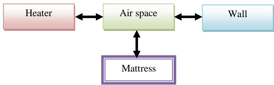
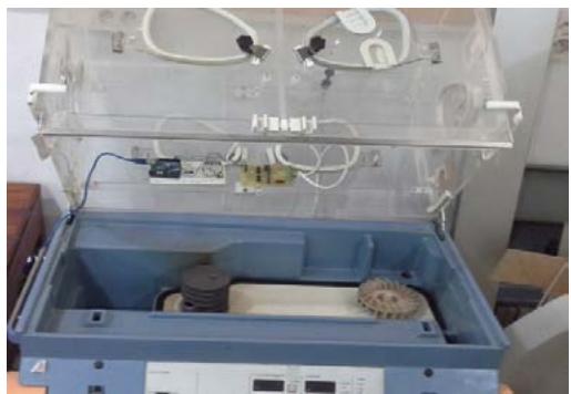DI = \left| Y_{i} \right\| e_{in} \bigg | + \left| Y_{s} \right| d

Figure 8: a) Compartments of the Closed Incubator System, b) Actual Image of the Incubator

6.2 Bond Graph Model

The incubator illustrated in figure 9 is modeled by the bond graph of figure 3 as follows:

★ The thermal capacity of an electrical resistor is modeled by a source of effort (Se: Te) with a capacitance (C: ) in series with a restriction ( );

★ The thermal capacity in the interior of the incubator by a capacitance (C: ) in series with a restriction ( );

★ The thermal capacity in the outside of the incubator by a capacitance (C: ) in series with a restriction ( );

★ The thermal capacity created by mattress by a capacitance (C: ) in series with a restriction ( );

★ The element (TF ) represents the thermal transformation between the thermal source and the internal volume of the incubator.

★ The element represents the thermal transformation between the thermal source and the mattress.

★ The external environment is modeled by a source of effort (Se: ) and restriction (R: Rex).

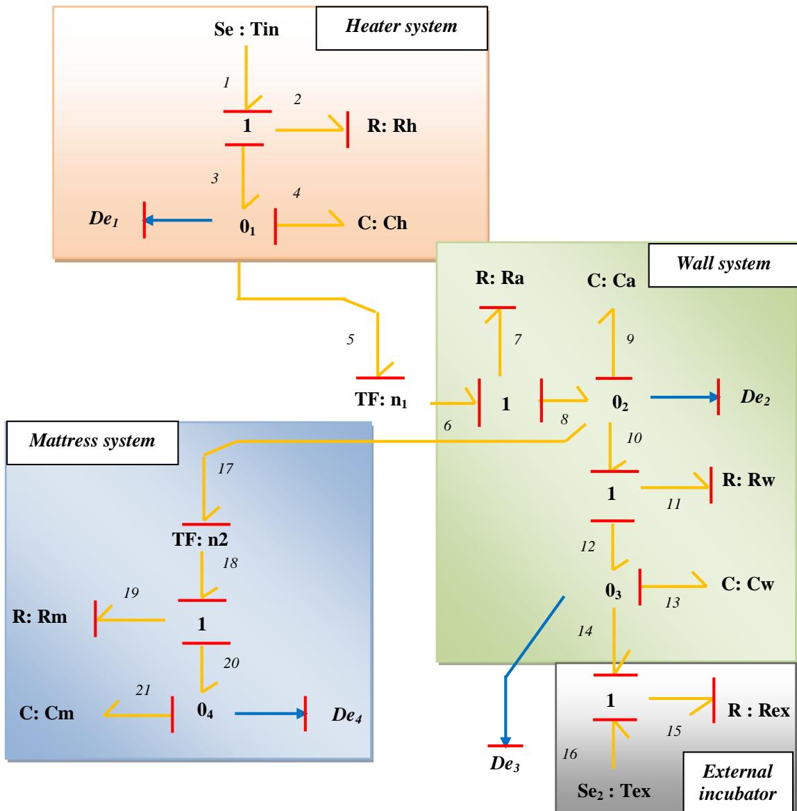Figure 9: Bond Graph model of Incubator Technology

6.3 Simulation Results of the Incubator

Figure 10 shows the evolution of temperature curves Th, Ta, Tw and Tm in the case of normal operation.

{"image_source":{"path":"images/5dd91e9d75d4d6a7a439ac27ae8076d2cce963d29b068964929e033fefce4347.jpg"},"content":"","chart_caption":[{"type":"text","content":"Time (s)"},{"type":"text","content":"Fig. 10: Evolution of Temperature Curves Th, Ta, Tw and Tm in the Case of Normal Operation"}],"chart_footnote":[]}

Determination of residue equations

◆ The junction gives us as equation:

r_{1}=f_{3}-f_{4}-f_{5}

According to these relations, one can deduce the residual equation :

r _ {1} = \frac{T _ {\text{inp}} - D e _ {1}}{R h} - C h. \frac{d D e _ {1}}{d t} - \frac{n _ {1} . \left(n _ {1} . D e _ {1} - D e _ {2}\right)}{R a}\tag{17}

◆ The junction gives us as equation:

r_{2}=f_{8}-f_{9}-f_{10}-f_{17}

According to these relations, one can deduce the residual equation :

r _ {2} = \frac{n _ {1} . D e _ {1} - D e _ {2}}{R a} - C a. \frac{d D e _ {2}}{d t} - \frac{n _ {2} . (n _ {2} . D e _ {2} - D e _ {"})}{R w} - \frac{n _ {3} . (n _ {3} . D e _ {2} - D e _ {3})}{R m}\tag{18}

◆ The junction gives us as equation:

r_{3} = f_{12} - f_{13} - f_{14}

According to these relations, one can deduce the residual equation :

r _ {3} = \frac{D e _ {2} - D e _ {3}}{R w} - C w \frac{d D e _ {3}}{d t} - \frac{D e _ {3} - T _ {e x}}{R _ {e x}}\tag{19}

◆ The junction gives us as equation:

r_{4} = f_{20} - f_{21}

According to these relations, one can deduce the residual equation :

r_{4} = \frac{n_{3}.(n_{3}.De_{2} - De_{4})}{Rm} - Cm\frac{dDe_{4}}{dt}

The default signature matrix is associated with the set of residues with the elements associated with the system . We denote the value M = 1 if the residual i is sensitive to this element, the opposite case M = 0, in the end we obtain the following signatures the table represented below. In our case, we have (4) four residues (17) seventeen elements.

Table 1: Fault Signatures Matrix for the Incubator

	$r_1$	$r_2$	$r_3$	$r_4$
$F_1: Tin$	1	0	0	0
$F_2: Tex$	0	0	1	0
$F_3: Ch$	1	0	0	0
$F_4: Ca$	0	1	0	0
$F_5: Cw$	0	0	1	0
$F_6: Cm$	0	0	0	1
$F_7: Rh$	1	0	0	0
$F_8: Ra$	1	1	0	0
$F_9: Rw$	0	0	1	0
$F_{10}: Rm$	0	1	0	1
$F_{11}: Rp$	0	0	1	0
$F_{12}: n_1$	1	1	0	0
$F_{13}: n_2$	0	1	0	1
$F_{14}: De_1$	1	1	0	0
$F_{15}: De_2$	1	1	1	1
$F_{16}: De_3$	0	1	1	0
$F_{17}: De_4$	0	1	0	1

{"image_source":{"path":"images/925ac0b143dda49cb30e8a4b179ca6da96c709f8c5638efc69aaca8e8a8ff26f.jpg"},"content":"","chart_caption":[{"type":"text","content":"Figure 11 shows the evolution of residues "},{"type":"equationinline","content":"r\{1}"},{"type":"text","content":", "},{"type":"equationinline","content":"r\{2}"},{"type":"text","content":", "},{"type":"equationinline","content":"r\{3}"},{"type":"text","content":" and "},{"type":"equationinline","content":"r\{4}"},{"type":"text","content":" as a normal function. The pitches of the residues converge towards zero under normal operating conditions."},{"type":"text","content":"Fig. 11: Evolution of Residues "},{"type":"equationinline","content":"r\{1}"},{"type":"text","content":", "},{"type":"equationinline","content":"r\{2}"},{"type":"text","content":", "},{"type":"equationinline","content":"r\{3}"},{"type":"text","content":" and "},{"type":"equationinline","content":"r\{4}"},{"type":"text","content":" in the Case of Normal Operation"}],"chart_footnote":[]}

6.4 Simulation Incubator With Faults

Fault on the Thermal Source

When a fault occurs on the heat source (damage to the heating resistance of the incubator) at the time t = 12000s, we find that:

★ All the residues , , and have non-zero average values, these residues are therefore sensitive to this defect, which is confirmed, by the theoretical results presented in table 2 (see Figure 12).

★ Temperatures Th, Ta, Tw and Tm suffered declines in their speed at the moment of failure (see Figure 13).

{"image_source":{"path":"images/f43cadbba49a7b728d050f1b257c947a9e817420437fa2d1c7a87576d2da4ce8.jpg"},"content":"","chart_caption":[],"chart_footnote":[]} {"image_source":{"path":"images/721afd15e3df05cc6a37d6ec82dea62431cf325d4eeb611d0edaf8efb2c196d3.jpg"},"content":"","chart_caption":[{"type":"text","content":"Fig. 12: Evaluation Of Residues "},{"type":"equationinline","content":"r\{1}"},{"type":"text","content":", "},{"type":"equationinline","content":"r\{2}"},{"type":"text","content":", "},{"type":"equationinline","content":"r\{3}"},{"type":"text","content":" and "},{"type":"equationinline","content":"r\{4}"},{"type":"text","content":" in the Case of a Fault on the Thermal Source"},{"type":"text","content":"Fig. 13: Evaluation of temperatures Th, Ta, Tw and Tm in the case of a fault on the thermal source. Fault inside the incubator"}],"chart_footnote":[]}

When a fault occurs on the incubator (open door of the incubator) at the time t = 17000s, we find that:

★ The residues r1, r2, r3 and r4 have non-zero average values, these residues are therefore sensitive to this defect, which is confirmed, by the theoretical results presented in table 2 (see Figure 14).

★ Temperatures Th, Ta, Tw and Tm suffered declines in their speed at the moment of failure (see Figure 15).

{"image_source":{"path":"images/821af04dc8dadd1e1db280293d19e44884541fe0b31c2b464791692586caa463.jpg"},"content":"","chart_caption":[{"type":"text","content":"Fig. 14: Evaluation of Residues "},{"type":"equationinline","content":"r\{1}"},{"type":"text","content":", "},{"type":"equationinline","content":"r\{2}"},{"type":"text","content":", "},{"type":"equationinline","content":"r\{3}"},{"type":"text","content":" and "},{"type":"equationinline","content":"r\{4}"},{"type":"text","content":" in the Case of Default in Inside the Incubator"}],"chart_footnote":[]} {"image_source":{"path":"images/3fdf7520f91670e34f47a845ac0ae2fb60ae4cfa147bd84cf78a952246153d9a.jpg"},"content":"","chart_caption":[{"type":"text","content":"Fig. 14: Evaluation of Temperatures Th, Ta, Tw and Tm in the Case of Default in Inside the Incubator"}],"chart_footnote":[]}

VII. ROBUST DIAGNOSIS BY BOND GRAPHS

7.1 BG-LFT Model of the Incubator Flawless

Figure 16 shows the BG-LFT model of the incubator system flawless. To determine the residues, we must put the system in the form derivative and also put sensors under dialyzed.

Determination of residues flawless

★ The junction gives us as equation:

R_{d1} = f_3 - f_4 - f_5 + w_{Ch} + w_{1/Rh} + w_{1/Ra}

From this relation, we can deduce the residual equation :

Rd_{1} = \frac{T_{inp}-De_{1}}{Rh} - Ch.\frac{dDe_{1}}{dt} - \frac{n_{1}.(n_{1}.De_{1}-De_{2})}{Ra} + w_{Ch} + w_{\frac{1}{Rh}} + w_{\frac{1}{Ra}}

The equation consists of two parts: the first part is the normal evolution of the residual and the second part represents the residual uncertainty related to the evolution of the parameters :

\left\{ \begin{array}{l} R d_{1} = r_{1 n} + d_{1} \\ r_{1 n} = \frac{T_{\text{inp}} - D e_{1}}{R h} - C h \cdot \frac{d D e_{1}}{d t} - \frac{n_{1} \cdot (n_{1} \cdot D e_{1} - D e_{2})}{R a} \\ d_{1} = w_{C h} + w_{\frac{1}{R h}} + w_{\frac{1}{R a}} + w_{\frac{1}{R w}} \end{array} \right.

★ The junction gives us as equation:

R d _ {2} = r _ {2} = f _ {8} - f _ {9} - f _ {1 0} - f _ {1 7} + w _ {C a} + w _ {1 / R a} + w _ {1 / R w}

From this relation, we can deduce the residual equation :

Rd_{2} = Ca.\frac{dDe_{2}}{dt} - \frac{De_{1}-De_{2}}{Ra} - \frac{De_{1}-De_{3}}{Rw} + w_{Ca} + w_{\frac{1}{Ra}} + w_{\frac{1}{Rw}}

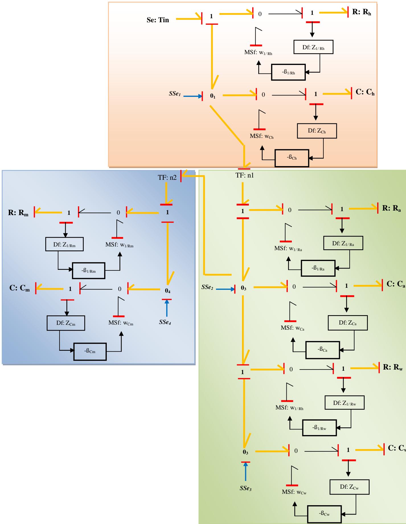Fig. 16: GB-LFT Approach Incubator System with Derivative Mode

The equation consists of two parts: the first part is the normal evolution of the residual and the second part represents the residual uncertainty related to the evolution of the parameters :

\left\{ \begin{array}{l} R d_{1} = r_{1 n} + d_{1} \\ r_{1 n} = \frac{T_{\text{inp}} - D e_{1}}{R h} - C h \cdot \frac{d D e_{1}}{d t} - \frac{n_{1} \cdot (n_{1} \cdot D e_{1} - D e_{2})}{R a} \\ d_{1} = w_{C h} + w_{\frac{1}{R h}} + w_{\frac{1}{R a}} + w_{\frac{1}{R w}} \end{array} \right.

★ The junction gives us as equation:

R d _ {2} = r _ {2} = f _ {8} - f _ {9} - f _ {1 0} - f _ {1 7} + w _ {C a} + w _ {1 / R a} + w _ {1 / R w}

From this relation, we can deduce the residual equation :

Rd_{2} = Ca.\frac{dDe_{2}}{dt} - \frac{De_{1}-De_{2}}{Ra} - \frac{De_{1}-De_{3}}{Rw} + w_{Ca} + w_{\frac{I}{Ra}} + w_{\frac{I}{Rw}}

The equation consists of two parts: the first part is the normal evolution of the residual and the second part represents the residual uncertainty related to the evolution of the parameters :

\left\{ \begin{array}{l} R d _ {2} = r _ {2 n} + d _ {2} \\ r _ {2 n} = \frac {n _ {1} . D e _ {1} - D e _ {2}}{R a} - C a. \frac {d D e _ {2}}{d t} - \frac {D e _ {1} - D e _ {3}}{R w} \\ - \frac {n _ {2} . (n _ {2} . D e _ {2} - D e _ {4})}{R m} \\ d _ {2} = w _ {C a} + w _ {\frac {1}{R a}} + w _ {\frac {1}{R w}} + w _ {\frac {1}{R m}} \end{array} \right.

★ The junction gives us as equation:

R d _ {3} = f _ {1 2} - f _ {1 3} - f _ {1 4} + w _ {C w} + w _ {1 / R w} + w _ {1 / R p}

From this relation, we can deduce the residual equation :

Rd_{3} = \frac{De_{2}-De_{3}}{Rw} - Cw\frac{dDe_{3}}{dt} - \frac{De_{3}-T_{ex}}{Rp} + w_{Cw} + w_{\frac{1}{Rw}} + w_{\frac{1}{Rp}}

The equation consists of two parts: the first part is the normal evolution of the residual and the second part represents the residual uncertainty related to the evolution of the parameters :

\left\{ \begin{array}{l} R d_{3} = r_{3 n} + d_{3} \\ r_{3 n} = \frac{D e_{2} - D e_{3}}{R w} - C w \frac{d D e_{3}}{d t} - \frac{D e_{3} - T_{e x}}{R p} \\ d_{3} = w_{C w} + w_{\frac{1}{R w}} + w_{\frac{1}{R p}} \end{array} \right.

★ The junction gives us as equation:

R d _ {4} = f _ {2 0} - f _ {2 1} + w _ {C m} + w _ {1 / R m}

According to these relations, one can deduce the residual equation :

Rd_{4} = \frac{n_{2}.(n_{2}.De_{2}-De_{4})}{Rm} - Cm\frac{dDe_{4}}{dt} + w_{Cm} + w_{1/Rm}

The equation consists of two parts: the first part is the normal evolution of the residual and the second part represents the residual uncertainty related to the evolution of the parameters :

\left\{ \begin{array}{l} R d_{4} = r_{4 n} + d_{4} \\ r_{4 n} = \frac{n_{2} \cdot (n_{2} \cdot D e_{2} - D e_{4})}{R m} - C m \frac{d D e_{4}}{d t} \\ d_{4} = w_{C m} + w_{1 / R m} \end{array} \right.

7.2: BG-LFT Model of the Incubator with Faults

Figure 17 shows the BG-LFT model of incubator system with defaults. We have introduced seven faults, four parametric faults ( , , , and ) and two structural faults ( and ).

Determination of residues with faults

★ The junction gives us as equation:

R _ {d 1} = f _ {3} - f _ {4} - f _ {5} + w _ {1}

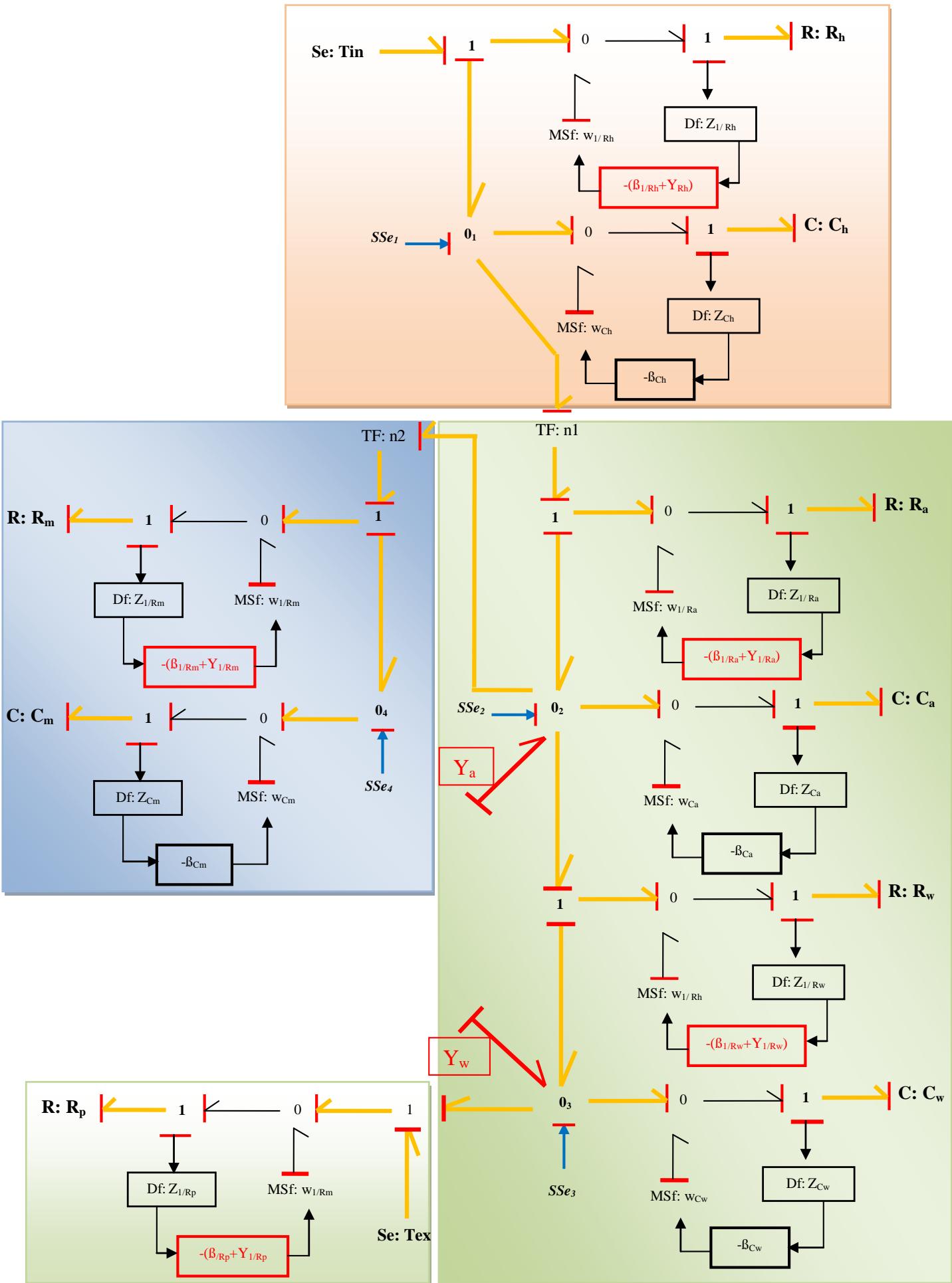Fig. 17: BG-LFT Approach Incubator System With Derivative Mode and Four Parametric Faults (YRh, YRa,, YRw, and YRm) and Two Structural Faults (Ya and Yw)

According to these relations, one can deduce the residual equation :

R d _ {1} = \frac{T _ {\text{inp}} - D e _ {1}}{R h} - C h. \frac{d D e _ {1}}{d t} - \frac{n _ {1} . (n _ {1} . D e _ {1} - D e _ {2})}{R a} + w _ {1}\tag{25}

With:

The equation consists of two parts: the first part is the normal evolution of the residual and the second part represents the residual uncertainty related to the evolution of the parameters :

\left\{ \begin{array}{l} R d_{1} = r_{1 n} + d_{1} \\ r_{1 n} = \frac{T_{\text{inp}} - D e_{1}}{R h} - C h \cdot \frac{d D e_{1}}{d t} - \frac{n_{1} \cdot (n_{1} \cdot D e_{1} - D e_{2})}{R a} \\ d_{1} = w_{1} \end{array} \right.

★ The junction gives us as equation:

R d _ {2} = f _ {8} - f _ {9} - f _ {1 0} + w _ {2}

According to these relations, one can deduce the residual equation :

With:

The equation consists of two parts: the first part is the normal evolution of the residual and the second part represents the residual uncertainty related to the evolution of the parameters :

Rd_{2}=Ca.\frac{dDe_{2}}{dt}-\frac{De_{1}-De_{2}}{Ra}-\frac{De_{1}-De_{3}}{Rw}+w_{2}

\left\{ \begin{array}{l} R_{2} = r_{21n} + d_{2} \\ r_{2n} = C a \cdot \frac{d D e_{2}}{d t} - \frac{D e_{1} - D e_{2}}{R a} - \frac{D e_{1} - D e_{3}}{R w} \\ d_{2} = w_{2} \end{array} \right.

★ The junction gives us as equation:

Rd_{3} = f_{12} - f_{13} + w_{3}

According to these relations, one can deduce the residual equation :

Rd_{3} = \frac{De_{2}-De_{3}}{Rw} - Cw\frac{dDe_{3}}{dt} - \frac{De_{3}-Tex}{Rp} + w_{3}

With:

The equation consists of two parts: the first part is the normal evolution of the residual and the second part represents the residual uncertainty related to the evolution of the parameters :

\left\{ \begin{array}{l} R d_{3} = r_{3 n} + d_{3} \\ r_{3 n} = \frac{D e_{2} - D e_{3}}{R w} - C w \frac{d D e_{3}}{d t} - \frac{D e_{3} - T e x}{R p} \\ d_{3} = w_{3} \end{array} \right.

★ The junction gives us as equation:

Rd_{4} = f_{20} - f_{21} + w_{4}

According to these relations, one can deduce the residual equation :

Rd_4 = \frac{n_2.(n_2.De_2 - De_4)}{Rm} - Cm\frac{dDe_4}{dt} + w_4

With:

The equation consists of two parts: the first part is the normal evolution of the residual and the second part represents the residual uncertainty related to the evolution of the parameters :

\left\{ \begin{array}{l} R d_{4} = r_{4 n} + d_{4} \\ r_{4 n} = \frac{D e_{1} - D e_{4}}{R m} - C m \frac{d D e_{4}}{d t} \\ d_{4} = w_{4} \end{array} \right.

VIII. PERFORMANCE INDICES FOR INCUBATOR

8.1: Sensitivity Index (SI)

Residue :

\left\{ \begin{array}{l} S I _ {1} = \frac {w _ {1}}{d _ {1}} \\ S I _ {2} = \frac {w _ {\frac {1}{R h}} + w _ {\frac {1}{R a}} + w _ {C h} + Y _ {\frac {1}{R h}} . f _ {h} + Y _ {\frac {1}{R a}} . f _ {a}}{d _ {2}} \end{array} \right. \tag{29}

Residue :

\left\{ \begin{array}{l} S I _ {2} = \frac {w _ {2}}{d _ {2}} \\ S I _ {2} = \frac {w _ {\frac {1}{R a}} + w _ {\frac {1}{R w}} + w _ {\frac {1}{R m}} + w _ {C a} + Y _ {\frac {1}{R a}} . f _ {a} + Y _ {\frac {1}{R w}} . f _ {w} + Y _ {\frac {1}{R m}} . f _ {m} + Y _ {a}}{d _ {2}} \end{array} \right. \tag{30}

Residue :

\left\{ \begin{array}{l} S I _ {3} = \frac {w _ {3}}{d _ {3}} \\ S I _ {3} = \frac {w _ {\frac {1}{R w}} + w _ {\frac {1}{R p}} + w _ {C w} + Y _ {\frac {1}{R w}} . f _ {w} + Y _ {\frac {1}{R w}} . f _ {w} + Y _ {w}}{\text{■Residue} R d _ {4} : d _ {3}} \end{array} \right. \tag{31}

Residue :

\left\{ \begin{array}{l} S I _ {4} = \frac {w _ {4}}{d _ {4}} \\ S I _ {4} = \frac {w _ {\frac {1}{R m}} + w _ {C m} + Y _ {\frac {1}{R m}} . f _ {m}}{d _ {1}} \end{array} \right. \tag{32}

8.2. Detectability index (DI)

Residue :

In this way, the defect detectability index of the residue is obtained:

DI_{1}=w_{1}-d_{1}

If then

\left\{ \begin{array}{l} w _ {1} \rangle d _ {1} \\ w _ {\frac {1}{R h}} + w _ {\frac {1}{R a}} + w _ {C h} + Y _ {\frac {1}{R h}}. f _ {h} + Y _ {\frac {1}{R a}}. f _ {a} \rangle d _ {1} \end{array} \right.\tag{37}

The detectable rate of a defect on the element is calculated by supposing

Y_{1/Ra}=0

\frac{Y_{\frac{1}{Rh}} \cdot \frac{d_1 - (w_{\frac{1}{Rh}} + w_{\frac{1}{Ra}} + w_{Ch})}{f_h}}

The detectable rate of a defect on the element is calculated by supposing

Y_{1/Rh}=0

\frac {Y _ {\frac {1}{R a}} \rangle \frac {d _ {1} - (w _ {\frac {1}{R h}} + w _ {\frac {1}{R a}} + w _ {C h})}{f _ {a}}}

Residue :

In this way, the defect detectability index of the residue is obtained:

D I _ {2} = w _ {2} - d _ {2}

If then

\left\{ \begin{array}{l} w_{2} \rangle d_{2} \\ w_{\frac{1}{R a}} + w_{\frac{1}{R w}} + w_{\frac{1}{R m}} + w_{C a} + Y_{\frac{1}{R a}}. f_{a} + Y_{\frac{1}{R w}}. f_{w} \\ + Y_{\frac{1}{R m}}. f_{m} + Y_{a}. f_{Y a} \rangle d_{2} \end{array} \right. \tag{38}

The detectable rate of a defect on the element is calculated by supposing

Y _ {1 / R w} = Y _ {1 / R m} = Y _ {a} = 0

\frac {Y _ {\frac {1}{R a}} \left\rangle \frac {d _ {2} - (w _ {\frac {1}{R a}} + w _ {\frac {1}{R w}} + w _ {\frac {1}{R m}} + w _ {C a})}{f _ {a}} \left. \right.}{}

The detectable value of a defect on the element is calculated assuming

Y _ {1 / R a} = Y _ {1 / R m} = Y _ {a} = 0

\frac {Y _ {\frac {1}{R w}} \left\rangle \frac {d _ {2} - (w _ {\frac {1}{R a}} + w _ {\frac {1}{R w}} + w _ {\frac {1}{R m}} + w _ {C a})}{f _ {w}} \left. \right.}{}

The detectable value of a defect on the element is calculated assuming

Y _ {1 / R a} = Y _ {1 / R w} = Y _ {a} = 0

\frac {Y _ {\frac {1}{R m}} \rangle \frac {d _ {2} - (w _ {\frac {1}{R a}} + w _ {\frac {1}{R w}} + w _ {\frac {1}{R m}} + w _ {C a})}{f _ {m}}}

The detectable value of the structural defect is calculated assuming

Y _ {1 / R m} = 0

Y _ {a} \rangle \frac {d _ {2} - w _ {\frac {1}{R a}} + w _ {\frac {1}{R w}} + w _ {\frac {1}{R m}} + w _ {C a}}{f _ {Y a}}

Residue :

In this way, the defect detectability index of the residue is obtained:

D I _ {3} = w _ {3} - d _ {3}\tag{34}

If >0 then

\left\{ \begin{array}{l} w _ {3} \rangle d _ {3} \\ w _ {\frac {1}{R w}} + w _ {\frac {1}{R p}} + w _ {C w} + Y _ {\frac {1}{R w}}. f _ {w} + Y _ {\frac {1}{R p}}. f _ {p} + Y _ {w}. f _ {Y w} \rangle d _ {3} \end{array} \right.

The detectable rate of a defect on the element is calculated by supposing

Y _ {1 / R p} = Y _ {w} = 0

\frac {Y _ {\frac {1}{R w}} \rangle}{d _ {3} - (w _ {\frac {1}{R w}} + w _ {\frac {1}{R p}} + w _ {C w})} {f _ {w}}

The detectable rate of a defect on the element is calculated by supposing

Y _ {1 / R w} = Y _ {w} = 0

\frac {Y _ {\frac {1}{R p}} \rangle}{d _ {3} - (w _ {\frac {1}{R w}} + w _ {\frac {1}{R p}} + w _ {C w})} f _ {p}

The detectable value of the structural defect is calculated assuming

\frac {Y _ {w} \left\rangle \frac {d _ {3} - (w _ {\frac {1}{R w}} + w _ {\frac {1}{R p}} + w _ {C w})}{f _ {Y w}} \left. \right.}{}

Residue :

In this way, the defect detectability index of the residue is obtained:

D I _ {4} = w _ {4} - d _ {4}\tag{40}

If >0 then

\left\{ \begin{array}{l} w _ {4} \rangle d _ {4} \\ w _ {\frac {1}{R m}} + w _ {C m} + Y _ {\frac {1}{R m}}. f _ {m} \rangle d _ {4} \end{array} \right.

The detectable rate of a defect on the element is calculated by the equation:

\frac {Y _ {\frac {1}{R m}} \left\rangle \frac {d _ {4} - (w _ {\frac {1}{R m}} + w _ {C m})}{f _ {m}} \left. \right.}{}

IX. CONCLUSION

In this paper, we presented diagnostic methods using the Bond Graph approach. The analytical redundancy relationships generated using the parity space method depends on the knowledge of the degree of derivations to be applied. The advantages of using the last method are: simplicity of understanding (ARRs) since they correspond to relationships and variables that are displayed by the leap graph model, and then the transition to the LFT form made by a simple addition of modulated sources of effort and flow on the model, image of the physical process, ARRs are deduced directly from the graphical representation, they can be generated in symbolic form and therefore adapted to a computer implementation.

ACKNOWLEDGEMENTS

We thank the National School of Engineers of Tunis, University of Tunis El Manar to support our work.

− Conflict of Interest

The authors declare no conflict of interest.

− Ethical Approval

Not applicable

− Data Availability

The datasets used in this study are openly available at [repository link] and the source code is available on GitHub at [GitHub link].

− Funding

This work did not receive any external funding.

− References

54 Cites in Article

REFERENCE FORMAT

− Cite this article

Generating citation...

Classification
1

LCC Code: T58.5
Version of record

v1.0
Issue date

17 January 2024
Language

en

Reliability of the Bond Graph Approach for Robust Diagnosis of a Newborn Incubator System

Download Article Access OJS

Open Access

Research Article

CC-BY-NC 4.0

LJER Volume 24 LJER Volume 24 Issue 1, Pg. 47-72

Explore Journal

Read LJER Volume 24 Issue 1 Explore LJER Volume 24

Views 613

Downloads 32

Year

Special Issue

Launch a focused special issue to highlight research, emerging trends, and expert insights in your academic field.

Keywords

5

analytical redundancy relations bond graph approach Incubator linear fractional transformations robust diagnosis

Reliability of the Bond Graph Approach for Robust Diagnosis of a Newborn Incubator System

IntelliPaper

Request Review Access

Order Article Reprints

− Abstract

− Explore Digital Article Text

I. INTRODUCTION

II. MATHEMATICAL MODEL OF THE INCUBATOR

2.1 Modeling the Thermostat

2.2 The Ambient Air in the Lodge

2.3 Thermal Balance of the Walls

2.4 Mattress Modeling

III. INDUSTRIAL SYSTEM BY BOND GRAPH MODELS

IV. ROBUST DIAGNOSIS OF INDUSTRIAL SYSTEM BY BOND GRAPH MODELS

4.1. Construction of a BG-LFT Model

4.3 Resistive Element With a Multiplicative Uncertainty

4.4 Storage Elements With a Multiplicative Uncertainty

4.5 Generation of Robust Residuals

V. ANALYSIS OF RESIDUALS SENSITIVITY

5.1 Sensitivity Index (SI)

5.2 Detectability Index (DI)

VI. MODELING AND SIMULATION RESULTS OF INCUBATOR BY BOND GRAPH MODELS

6.1 Incubator System

6.2 Bond Graph Model

6.3 Simulation Results of the Incubator

6.4 Simulation Incubator With Faults

VII. ROBUST DIAGNOSIS BY BOND GRAPHS

7.1 BG-LFT Model of the Incubator Flawless

7.2: BG-LFT Model of the Incubator with Faults

VIII. PERFORMANCE INDICES FOR INCUBATOR

8.1: Sensitivity Index (SI)

8.2. Detectability index (DI)

IX. CONCLUSION

ACKNOWLEDGEMENTS

− Conflict of Interest

− Ethical Approval

− Data Availability

− Funding

− References

− Cite this article

− Related Research

Classification

Version of record

Issue date

Language

Special Issue

Keywords

Next Research

Copy of Cardiovascular Risk Factors and Cardiovascular Risk in People Living with HIV: Comparison of Four Cardiovascular Risk Prediction Algorithms

Privacy preferences