Nonlinear Analysis as a Calculus

I. INTRODUCTION

There are two universal methods for local study of nonlinear equations and systems of different kinds (algebraic, ordinary and partial differential): (a) normal form and (b) truncated equations.

(a) Equations with linear parts can be reduced to their normal forms by local changes of coordinates. For algebraic equation, it is Implicit Function Theorem. For systems of ordinary differential equations (ODE), I completed the theory of normal forms, began by Poincaré (1879) [Poincaré, 1928] and Dulac (1912) [Dulac, 1912] for general systems [Bruno, 1964; 1971] and began by Birkhoff (1929) [Birkhoff, 1966] for Hamiltonian systems [Bruno, 1972; 1994].

(b) Equations without linear part: I proposed to study properties of solutions to equations (algebraic, ordinary differential and partial differential) by studying sets of vector power exponents of terms of these equations. Namely, to select more simple ("truncated") equations [Bruno, 1962; 1989; 2000] by means of generalization to polyhedrons the Newton (1678) [Newton, 1964] and the Hadamard (1893) [Hadamard, 1893] polygons.

By means of power transformations [Bruno, 1962; 1989; 2022b] the normal forms and the truncated equations can be strongly simplified and often solved. Solutions to the truncated equations are asymptotically the first approximations of the solutions to the full equations. Continuing that process, we can obtain approximations of any precision to solutions of initial equations. Basing on the developed Asymptotic and Local Nonlinear Analysis, I proposed algorithms for solutions of a wide set of singular problems. In particular, for computation of six different types of asymptotic expansions of solutions to ODE [Bruno, 2004; 2018b; Bruno, Goruchkina, 2010], including expansions into trans-series [Bruno, 2019b].

In this article it is shown for a single algebraic equation in Section 2, for a single ordinary differential equation in Section 3, for an autonomous system of ODE's in Section 4, for Hamiltonian system in Subsection 4.5, for a single partial differential equation in Section 5. A survey of some applications is in Section 6.

From that point of view, the usual Classical Analysis is linear one, because it considers only linear approximations of problems near known solutions.

II. SINGLE ALGEBRAIC EQUATION

2.1. The implicit function theorem: Let , , then

Theorem 2.1. Let

where , , the sum is finite and are some functions of , besides , . Then the solution to the equation has the form

where , , the coefficients are functions on T that are polynomials from with divided by . The expansion is unique. Let

then .

This is a generalization of Theorem 1.1 of [Bruno, 2000, Ch. II] on the implicit function and simultaneously a theorem on reducing the algebraic equation (2.1) to its normal form (2.2) when the linear part is nondegenerate. In it, we must exclude the values of near the zeros of the function .

Let or , and be a polynomial. A point , is called simple if the vector in it is non-zero. Otherwise, the point is called singular or critical. By shifting we move the point to the origin . If at this point the derivative , then near all solutions to the equation have the form , that is, lie in -dimensional space.

2.2. Newton's polyhedron: Let the point be singular. Write the polynomial in the form

where , or . Let .

The set S is called the support of the polynomial . Let it consist of points . The convex hull of the support is the set

which is called Newton's polyhedron.

Its boundary consists of generalized faces , where is its dimension of and is the number.

Each (generalized) face corresponds to its:

• boundary subset

• truncated polynomial

• and normal cone

where , the space is conjugate (dual) to the space and is the scalar product.

At solutions to the full equation tend to non-trivial solutions of those truncated equations whose normal cone intersects with the negative orthant in .

Remark 1. If in the sum (2.1) all belong to a forward cone :

then in the solution (2.2) of Theorem 2.1 all belong to the same cone : , , [Bruno, 1989, Part I, Chapter 1, § 3].

2.3. Power transformations [Bruno, 1962; 2000:] Let . The linear transformation of the logarithms of the coordinates

where is a nondegenerate square n-matrix, is called power transformation.

By the power transformation (2.5), the monomial transforms into the monomial , where and the asterisk indicates a transposition.

A matrix is called unimodular if all its elements are integers and . For an unimodular matrix , its inverse and transpose are also unimodular.

Theorem 2.2. For the face there exists a power transformation (2.5) with the unimodular matrix which reduces the truncated sum to the sum from coordinates, that is, , where is a polynomial. Here . The additional coordinates are local (small).

The article [Bruno, Azimov, 2023] specifies an algorithm for computing the unimodular matrix of Theorem 2.2.

2.4. Parametric expansion of solutions: Let be a face of the Newton polyhedron . Let the full equation is changed into the equation after the power transformation of Theorem 2.2. Thus .

Let the polynomial be the product of several irreducible polynomials

where . Let the polynomial be one of them. Three cases are possible:

Case 1. The equation has a polynomial solution . Then in the full polynomial let us substitute the coordinates

for the resulting polynomial again construct the Newton polyhedron, separate the truncated polynomials, etc. Such calculations were made in [Bruno, Batkhin, 2012] and were shown in [Bruno, 2000, Introduction].

Case 2. The equation has no polynomial solution, but has a parametrization of solutions

Then in the full polynomial g Y (we)substitute the coordinates

where and from the full polynomial we get the polynomial

where , , . Thus , .

If in the expansion (5.7) , then . By Theorem 2.1, all solutions to the equation have the form

i.e., according to (2.7) the solutions to the equation g = 0 have the form

Such calculations were proposed in [Bruno, 2018a].

If in (5.7) , then in (2.8) and for the polynomial (2.8) from , we construct a Newton polyhedron by support , separate the truncations and so on.

Case 3. The equation has neither a polynomial solution nor a parametric one. Then, using Hadamard's polyhedron [Bruno, 2018a; 2019a], one can compute a piece-wise approximate parametric solution to the equation and look for an approximate parametric expansion.

Similarly, one can study the position of an algebraic manifold in infinity.

III. SINGLE ODE [BRUNO, 2004]

3.1. Setting of the problem: Here we consider an ordinary differential equation of the form

where x is independent variable, y is the dependent variable, and f is a polynomial of its arguments. Near or we look for solutions of equation (3.1) in the form of asymptotic series

where are functions of and with

We set . By a differential monomial we mean the product of an ordinary monomial

is called a differential sum. In equation (3.1) polynomial f is the differential sum.

To every differential monomial one assigns its (vector) exponent by the following rules. For a monomial of the form (3.4) let

that is, ; for a derivative of the form (3.5) let

When differential monomials are multiplied, their exponents are summed as vectors:

The set of exponents of all the differential monomials in a differential sum of the form (3.6) is called the support of the sum . Obviously, . The closure of the convex hull of the support is referred to as the polygon of the sum . The boundary of the polygon consists of vertices and edges . These objects are called (generalized) faces , where the superscript indicates the dimension of the face and the subscript is the number of the face. Corresponding to any face are the related boundary subset of the set S and the truncated sum

Let be the plane conjugate to the plane so that the inner (scalar) product

is defined for any and . Corresponding to any face are its normal cone,

and the truncated sum (3.7).

All these constructions are applicable to equation (3.1), where is a differential sum.

Let or and suppose that a solution of the equation (3.1) has the form

where is a coefficient, , , the exponents r and are in R, and . Then we say that the expression

gives the power-law asymptotic form of the solution (3.8).

Thus, corresponding to any face are the normal cone in and the truncated equation

Theorem 3.1 ([Bruno, 2000, Chap. VI, Theorem 1.1]). If the equation (3.1) has a solution of the form (3.8) and if , then the truncation (3.9) of the solution (3.8) is a solution of the truncated equation (3.7), (3.10).

Therefore, to find all truncated solutions (3.9) of the equation (3.1), one must calculate the support , the polygon , all its faces , the outward normals to the edges , the normal cones of the edges, and the normal cones of the vertices. For each truncated equation (3.7), (3.10) one must then find all its solutions of the form (3.9) such that the vector belongs to , and single out the solutions of this kind for which one of the vectors belongs to the normal cone . If d=0, then one of the vectors belongs to . If d=1, then this property always holds. Here the value of is also determined.

3.2. Solution of the truncated equation: Here we consider separately two cases: a vertex and an edge . Corresponding to a vertex is a truncated equation (3.10) with one-point support Q and with d = 0. We set . Then the solution (3.7), (3.10) satisfies the equation

Substituting into , we see that does not depend on x, c and is a polynomial in r, that is,

where is the characteristic polynomial of the differential sum . Hence, in a solution (3.9) of the equation (3.10) the exponent r is a root of the characteristic equation

and the coefficient is arbitrary. Among the roots of the equation (3.11), one must single out only those for which one of the vectors , where , belongs to the normal cone of the vertex . In this case the value of uniquely determined. The corresponding expressions of the sum with an arbitrary constant are candidates for the role of truncated solutions of the equation (3.1). Moreover, by (3.3), if , then , and if , then .

Complex roots r to characteristic equation (3.11) may bring to exotic expansions of solutions (3.2), where coefficients are power series in with real and .

Corresponding to an edge is a truncated equation (3.10) with d=1 whose normal cone is a ray . If , this condition uniquely determines the exponent r of the truncated solution (3.9) and the value in (3.3). To find the coefficient , one must substitute the expression (3.9) into the truncated equation (3.10). After cancelling a factor which is a power of x, we obtain an algebraic defining equation for the coefficient ,

Corresponding to every root of this equation is an expression of the form (3.9) which is a candidate for the role of a truncated solution of the equation (3.1). Moreover, by (3.3), if in the normal cone one has , then , and if , then .

Thus, every truncated equation (3.10) has several suitable solutions of the form (3.9). Let us combine these solutions into families that are continuous with respect to , and the parameters of the equation (3.1) and denote these families by , where

If in the truncated equation (3.10), we make the power transformation

and the logarithmic transformation

then we obtain ODE

where is a differential sum, i.e. it has the form (3.1). If the equation (3.12) has a solution in the form

then in the expansion (3.2) coefficients are functions from . If , then it is the power-logarithmic expansion, where other are polynomials in . If depends on , then all are power series in and the expansion (3.2) is complicated.

3.3. Computation of solution to equation (3.1) as expansion (3.2)

From the polygon of the initial equation (3.1) we take a vertex or an edge . Then we found a power solution of the truncated equation , as it was described above, put

and obtain new equation

We construct the polygon for the new equation, take a vertex or an edge , solve the truncated equation

and obtain the second term of expansion (3.2) and so on.

We construct the polygon for the new equation, take a vertex or an edge , solve the truncated equation

and obtain the second term of expansion (3.2) and so on.

In [Bruno, 2004] there are some properties, that simplify computation.

Thus, we can obtain the 4 types of expansions (3.2) of solutions to equation (3.1):

1. Power, when all [Ibid.];

2. Power-logarithmic, when const and other are polynomial in log [Ibid.];

3. Complicated, when all are power series in [Bruno, 2006; 2018b];

4. Exotic, when all are power series in [Bruno, 2007].

Except expansions (3.2) of solutions of equation (3.1), there are exponential expansions

where and are power series in [Bruno, 2012a,b].

Also there are solutions in the form of transseries [Bruno, 2019b].

These results were applied to 6 Painlevè equations [Bruno, 2015; 2018b,c; Bruno, Goruchkina, 2010].

Written as differential sums they are:

Equation :

Equation :

Equation : .

Equation : .

Equation :

Equation :

Here a, b, c, d and , , , are complex parameters. If all they are nonzero, then polygons for these equations are shown in Figures 1, 2, 3.

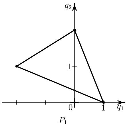
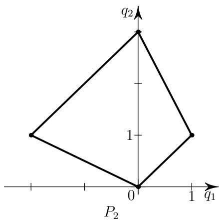Figure 1: Supports and polygons for equations
(left), (right).

3.4. Normal form: Roots of the equation (3.11) are called as eigenvalues of the differential sum , corresponding to the vertex. If the differential sum has order l, then the characteristic equation (3.11) has l roots, .

Theorem 3.2. Let

1. be a polynomial in ;

2. its polygon have a vertex at the left side of its boundary ;

3. truncated differential sum have eigenvalues , ;

4. the most left point of the support in the axis be . Evidently .

Then there exists such power series with integral increasing exponents, that after substitution

the transformed differential sum

for

has only resonant terms , where

and .

So here the eigenvalue is resonant if .

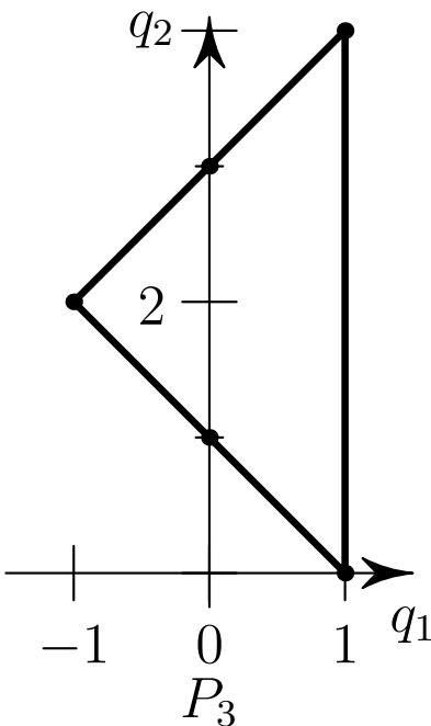
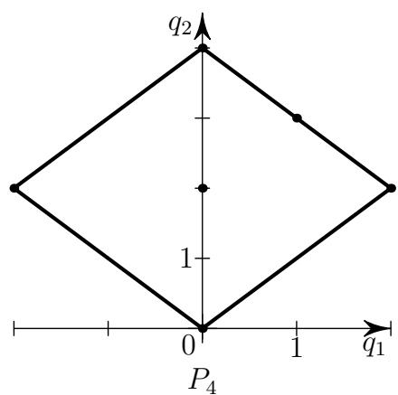Figure 2: Supports and polygons for equations
(left), (right).

Theorem 3.3. Let

1. be a polynomial in ;

2. its Newton polygon have a vertex at the right side of its boundary ;

3. truncated differential sum have eigenvalues , ;

4. the most right point of the support in the axis be . Evidently .

Then there exists such power series with integral decreasing exponents, that after substitution (3.13), the differential sum (3.14) for identities (3.15) has only resonant terms , where equality (3.16) is true, and .

So here the eigenvalue is resonant if . Equations for (3.14) in situations of Theorems 3.2 and 3.3 we will call normal forms.

Corollary 3.3.1. If the truncated sum has no integral eigenvalue (for Theorem 3.2) or (for Theorem 3.3), then the initial equation has formal solution . If the truncated sum contains the derivation , then the series converges according to Theorem 3.4 in [Bruno, 2004].

Remark 2. If the truncated sum has integral eigenvalue (for Theorem 3.2) or (for Theorem 3.3), then the initial equation

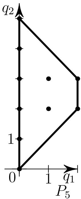
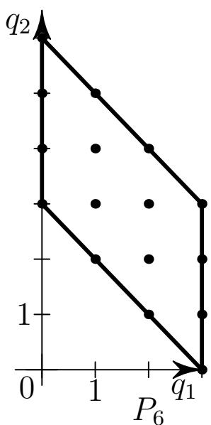Figure 3: Supports and polygons for equations
(left), (right).

3.5. Space Power Geometry: We will consider such a generalization of the power function which preserves their main properties. The real number

where , is called the order of the function on the ray when or . The order is not defined on the ray , where the limit point x = 0 or is a point of accumulation of poles of the function .

In Subsections 3.2-3.4 it was shown that as ( ) or as ( ) solutions to the ODE , where is a differential sum, can be found by means of algorithms of Plane PG, if

where n is the maximal order of derivatives in . Here we introduce algorithms, which allow calculate solutions with the property

where .

Lemma 3.3.1. If

then

Note, that in Plane PG we had , i.e. . So, new interesting possibilities correspond to .

We consider the ODE

where is a differential sum. To each differential monomial , we assign its (vector) power exponent by the following rules:

power exponent of the product of differential monomials is the sum of power exponents of factors: .

The set of power exponents of all differential monomials presented in the differential sum is called the space support of the sum . Obviously, . The convex hull of the support is called the polyhedron of the sum . The boundary of the polyhedron consists of the vertices , the edges and the faces . They are called (generalized) faces , where the upper index indicates the dimension of the face, and the lower one is its number. Each face corresponds to the space truncated sum

The approach allows to obtain solutions with expansions (3.2), where coefficients are all periodic or all elliptic functions [Bruno, 2012c,d; Bruno, Parusnikova, 2012].

Expansions of solutions to more complicated equations such as hierarchies Painlevé see in [Anoshin, Beketova, (et al.), 2023; Bruno, Kudryashov, 2009].

For Painlevé equations with all parameters nonzero, their polyhedrons are shown in Figures 4, 5, 6, 7, 8 correspondingly.

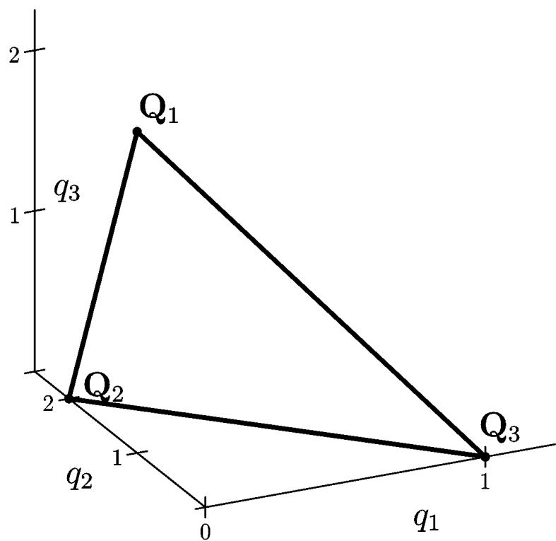Figure 4: Support and polyhedron for equation
.

IV. AUTONOMOUS ODE SYSTEM

Here we consider the system

where , or , all are polynomials from X. A point is called singular if all , .

4.1. Normal form: Let the point be a singular point. Then the system (4.1) has the linear part

where A is a square n-matrix. Let be a vector of its eigenvalues.

Theorem 4.1 ([Bruno, 1964; 1971, 1972]). There exists an invertible formal change of coordinates

where are power series from without free terms, which reduces the system (4.1) to normal form

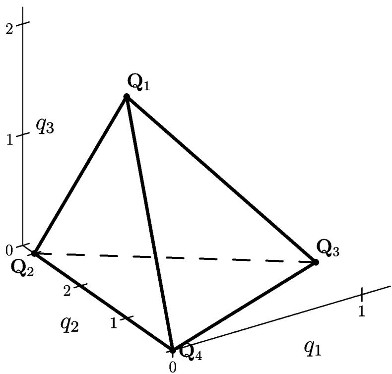Figure 5: Support and polyhedron for equation
.

containing only resonant terms , which have

Here are power series on Y without free terms.

and . Then the number k of linearly independent satisfying the equation (4.3) is called multiplicity of resonance.

Theorem 4.2. Let k be the multiplicity of resonance of the system (4.1). Then there exists a power transformation

with unimodular matrix which reduces the normal form (4.2), (4.3) to the system

in which the first k coordinates form a closed subsystem without a linear part, and the remaining n - k coordinates are expressed via them by means of integrals.

Thus, if , then the original system (4.1) of order n can be reduced to a system of order k, but without the linear part.

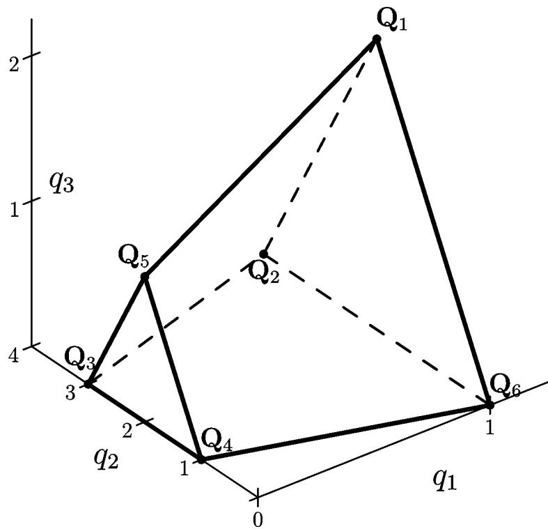Figure 6: Support and polyhedron for equation
.

4.2: Newton's polyhedron [Bruno, 1962; 2000]. Let's write the system (4.1) as

and put

The set

is called the support of the system (4.4). Its convex hull (2.3) is its Newton's polyhedron. Its boundary consists of generalized faces of dimensions , , and with numbers .

Each generalized face corresponds to:

• boundary subset ,

• truncated system

• normal cone (2.4) and

• tangent cone .

According to [Bruno, 2000, Chapt. 1, §2] let and be the interior point of a face , that is, does not lie in a face of smaller dimension. If , then . The conic hull of the set

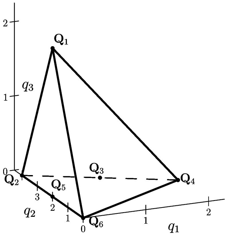Figure 7: Support and polyhedron for equation
.

is called the tangent cone of the face , , .

Theorem 4.3. For each generalized face , there exists power transformation

with the unimodular matrix and change of time

, which reduce the system (4.4) to the form

where the system

corresponds to the truncated system (4.5).

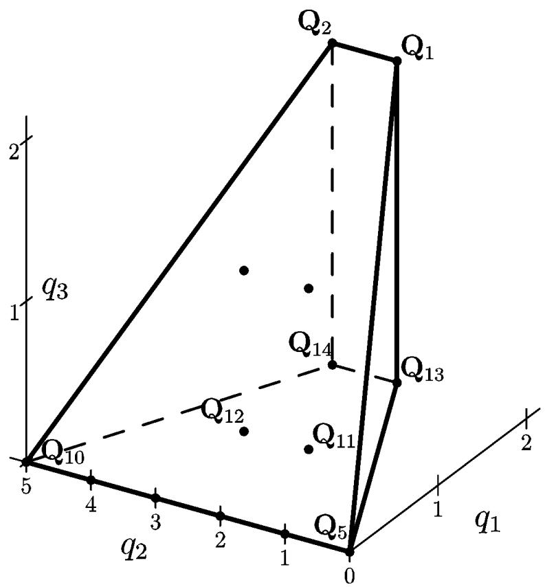Figure 8: Support and polyhedron for equation
.

If the face had normal and tangent cones and , then the truncated system (4.7) has normal and tangent cones and , which are obtained from and by conjugate linear transformations.

4.3. Generalized normal form [Bruno, 2022b]: Let the point

be singular for the truncated system (4.7). Near the point (4.8), the local coordinates are

Let at the point the eigenvalues of the matrix of the linear part of the system (4.7) are , where are the eigenvalues of the subsystem of the first d equations.

Theorem 4.4. There exists an invertible formal change of coordinates

where which reduces the system (4.6) to the generalized normal form

where

Here , where .

The system (4.9), (4.10) is reduced to a system of lower order by the power transformation of Theorem 4.2.

4.4. Analysis of singularities: Let be a singular point of the system tem (4.1). Two cases are possible:

Case 1. , then by Theorem 4.1 we reduce the system to a normal form, then by Theorem 4.2 we reduce the normal form to a subsystem of order k < n without linear part and obtain the problem of studying its singular points.

Case 2. , then we compute the Newton polyhedron and separate truncated systems in which the normal cone intersects the negative orthant of . Each of them is reduced to the form (4.6), (4.7) by the transformation of Theorem 4.3. For each singular point (4.8), we apply Theorem 4.4 and obtain a subsystem of smaller order.

Continuing this branching process, after a finite number of resolution of singularities we come to an explicitly solvable system from which we can understand the nature of solutions of the original system.

But Theorem 4.3 can be applied to the original system (4.1), i.e. to each of the generalized faces of its Newton polyhedron . Then to each singular point (4.8) we apply Theorems 4.4, 4.2 and reduce the order of the system. Here also through a finite number of steps of the singularity resolution we come to an explicitly solvable system. This allows us to study the singularities of the original system in infinity. This is the basis of the integrability criterion in [Bruno, Enderal, 2009; Bruno, Enderal, Romanovski, 2017].

The normal form can be computed in the neighborhood of a periodic solution or invariant torus [Bruno, 1972, II, §11], [Bruno, 2022a].

See [Bruno, Batkhin, 2023] for similar computations for a system of partial differential equations.

4.5. Hamiltonian system: It has the form

and is defined by one Hamiltonian function , where , . Here the normal form of the system (4.11) corresponds to the normal form of one Hamiltonian function. See details in [Bruno, Batkhin, 2021].

V. ONE PARTIAL DIFFERENTIAL EQUATION

5.1. Support [Bruno, 2000 Ch. 6-8]: Let or be independent variables and or be a dependent one. Consider .

Differential monomial is called a product of an ordinary monomial

where c = const, and a finite number of derivatives of the following form

Vector power exponent corresponds to the differential monomial , it is constructed according to the following rules:

The product of monomials corresponds to the sum of their vector power exponents:

Differential sum is the sum of differential monomials

If has no similar terms, then the set is called support of the sum (5.1).

5.2. Resonant monomials: Let the support of the differential sum (5.1) consists of one point . Then the substitution

in the differential sum gives the monomial

where is a polynomial of P which coefficients depend on P.

Monomial (5.2) will be called resonant for if for it

Let be the maximal order of the derivative over in , . If in

then

where is the characteristic polynomial of the sum of and its coefficients do not depend on P. But if the inequalities (5.3) are not satisfied, then .

Example. Let , .

Generally here for , we have and .

5.3. Normal form: For a differential sum we denote by the sum of all differential monomials of which have coordinate of vector power exponents equal to k: . Denote .

Consider the PDE

Theorem 5.1. Let

where all . Suppose

1. is a power series from X without a free term,

2. , where , .

Then there exists a substitution , where is a power series from X without a free term, which transforms the equation (5.4) to the normal form

where is a power series without a free term, containing only resonant monomials for sum .

Corollary 5.1.1. If the sum has no resonance monomials with , , then and

is the formal solution to the equation (5.4).

If in equation (5.4) differential sum does not contain derivatives, then

Hence has no resonant monomials and in the normal form (5.5) the series . So Theorem 5.1 gives the Implicit Function Theorem 2.1 without . If in Equation (5.4) , then Theorem 5.1 gives Theorem 3.2.

5.4. Polyhedron and truncated equations: Closure of a convex hull

of the support is called the polyhedron of sum . The boundary of the polyhedron consists of generalized faces , where . Each face corresponds to normal cone

where the space is conjugate to the space , is the scalar product, and truncated sum

Consider the equation

where f is the differential sum. In the solution of equation (5.6)

where is a series on the powers of and their logarithms, the series corresponds to its support, polyhedron, normal cones and truncations. The logarithm has a zero power exponent on . The truncated solution corresponds to the normal cone

Theorem 5.2. If the normal cone u intersects with the normal cone (5.2), then the truncation of the solution (5.3) satisfies the truncated equation

5.5. Power transformations: To simplify the truncated equation (5.8), it is convenient to use a power transformation. Let be a square real nondegenerate block matrix of dimension of the form

where and are square matrices of dimensions and 1, respectively. We denote , and by the asterisk * we denote transposition.

Variable change.

is called the power transformation.

Theorem 5.3 ([Bruno, 2000]). The power transformation (5.5) reduces a differential monomial with a power exponent into a differential sum with a power exponent :

Corollary 5.3.1. The power transformation (5.9) reduces the differential sum (2.1) with support to the differential sum with support , i.e.

Theorem 5.4. For the truncated equation

there is a power transformation (5.9) and monomial that translates the equation above into the equation

where is a differential sum whose support has zero coordinates.

5.6. Logarithmic transformation: Let be one of the coordinates or y. Transformation

is called logarithmic.

Theorem 5.5. Let be a differential sum such that all its monomials have a jth component of the vector exponent of degree equal to zero, then the logarithmic transformation (5.1) reduces the differential sum into a differential sum from .

5.7. Calculating asymptotic forms of solutions: A truncated equation

is taken. If it cannot be solved, then a power transformation of the Theorem 5.4 and then a logarithmic transformation of the Theorem 5.5 should be performed. Then a simpler equation is obtained. In case it is not solvable again, the above procedure is repeated until we get a solvable equation. Having its solutions, we can return to the original coordinates by doing inverse coordinate transformations. So the solutions written in original coordinates are the asymptotic forms of solutions to the original equation (5.2).

In [Bruno, Batkhin, 2023] method of selecting truncated equations was applied to systems of PDE.

Traditional approach to PDE see in [Oleinik, Samokhin, 1999; Polyanin, Zhurov, 2021].

VI. APPLICATIONS

Here we provide a list of some applications in complicated problems of (c) Mathematics, (d) Mechanics, (e) Celestial Mechanics and (f) Hydromechanics.

(c) In Mathematics: together with my students I found all asymptotic expansions of five types of solutions to the six Painlevé equations (1906) [Bruno, 2018c; Bruno, Goruchkina, 2010] and also gave very effective method of determination of integrability of ODE system [Bruno, Enderal, 2009; Bruno, Enderal, Romanovski, 2017].

(d) In Mechanics: I computed with high precision influence of small mutation oscillations on velocity of precession of a gyroscope [Bruno, 1989] and also studied values of parameters of a centrifuge, ensuring stability of its rotation [Batkhin, Bruno, (et al.), 2012].

(e) In Celestial Mechanics: together with my students I studied periodic solutions of the Beletsky equation (1956) [Bruno, 2002; Bruno, Varin, 2004], describing motion of satellite around its mass center, moving along an elliptic orbit. I found new families of periodic solutions, which are important for passive orientation of the satellite [Bruno, 1989], including cases with big values of the eccentricity of the orbit, inducing a singularity. Besides, simultaneously with [Hénon, 1997], I found all regular and singular generating families of periodic solutions of the restricted three-body problem and studied bifurcations of generated families. It allowed to explain some singularities of motions of small bodies of the Solar System [Bruno, Varin, 2007]. In particular, I found orbits of periodic flies round planets with close approach to the Earth [Bruno, 1981].

(f) In Hydromechanics: I studied small surface waves on a water [Bruno, 2000, Chapter 5], a boundary layer on a needle [Bruno, Shadrina, 2007], where equations of a flow have a singularity, and an one-dimensional model of turbulence bursts [Bruno, Batkhin, 2023].