





IntelliPaper
Abstract
In this contribution, we propose a single-species population growth model formulated using ideas emanating from Liebig’s principle of limiting factors. The inherent natural natality rate determines by the minimum between the size of the population and that of a resource on which the population depends for sustenance. Moreover, emulating the unrestricted population growth assumption, we hypothesise that the associating natural mortality rate is proportional to population size. We also consider that the external feeding resource's consumption rate varies directly proportional to the natural growth rate of the population. In this delivery, we present a qualitative study of the associated trajectories and fitting results based on data on populations growing under experimental or natural conditions. The possible phase configurations include regimes with stable equilibria, sigmoidal growth, extinction, or stationarity. All study cases confirmed that the offered model entails high reproducibility of observed variation patterns while supplying remarkable interpretative capabilities. The proposed model also allows simultaneous identification of the population size trajectory and the resource abatement function. One phase of Liebig’s limiting factors principle-driven model can consistently mimic population size abatement to extinction. Such a feature misses improved in regularly conceived S-shaped population growth models.
Explore Digital Article Text
I. INTRODUCTION
The optimal settings for biological processes often occur at the minimum and maximum values of relevant variables (Ghaleb et al., 2020; Peeters & Gardeniers, 1998). The concept of extreme value control ascended from results reported by K. Sprengel in 1839 (Sprengel, 1839; El-Sharkawy, 2011) and later popularised by Justus von Liebig, stating that the nutrient present in the minimum determines the rate of growth of a particular organism (Liebig, 1843). This observation led to the establishment of Liebig's Principle of Limiting Factors, also known as Liebig's Law of the Minimum (Rizhinashvili, 2022; Anees, 2022). Agents that slow down growth in an ecosystem constitute limiting factors. Control exerts by either the minimum or maximum values that the factor can assume over a gradient of variation. Based on lower and upper tolerance limits, Liebig's Law of the Minimum was generalised into the Law of the Tolerance of
Shelford (Shelford, 1913). Furthermore, limiting factors can indirectly influence the impact of other non-limiting factors by interacting with them. This principle, known as the principle of Limiting Factors, is treasured in studying the entire or parts of ecosystems (Odum,1963; Odum,1971).
Although in the ecological literature, the control by extreme values regularly cites, its utilisation as a conceptual framework for population growth models is limited. The initial effort to apply this concept was due to I. A. Polyetayev et al. in 1971, who proposed a Liebig's Principle of Limiting Factors-based model for predator-prey interactions (Polyetayev et al., 1971). In the Polyetayev model, the natality rate for the prey population determines by the minimum between the population size and the extent of an external resource representing feeding energy availability. Building upon these ideas, Echavarria and Gomez (1979) and Montiel-Arzate, et al. (2004) further developed related population models by maintaining natality as controlled by Liebig's Law of the Minimum but emulating Shelford's Law of Tolerance by hypothesising that the mortality rate regulates by the maximum value of factors depending on population size. Recently, Echavarria-Heras et al. (2021) revised the approach by Montiel-Arzate et al. (2004) to propose a model for the growth of a single species population built upon the Liebig-Shelford as mentioned earlier paradigm for the control of the related natural growth rate, but including a specific scaling or weighting of population size to model the increase in mortality promoted by low population densities. This last approach reported consistent reproducibility when fitted on real data sets. However, the authors also reported inconveniences since a direct fitting procedure that relies on estimates' initial values brought high sensibility associated with local minimum problems at the nonlinear acquisition of final values. Therefore, a revision aimed to avoid or at least lessen the parameter estimation burden experienced deems necessary. In that vein, reducing the complexity associated with the Echavarria-Heras et al. (2021) construct while simultaneously keeping its reproducibility strength endures a reasonable rationale. For that aim, in this contribution, we modify the protocol by Echavarria-Heras et al. (2021) and propose a single species population growth model, built upon Liebig's Principle of Limiting Factors and such that: (1) the inherent natural natality rate is determined according to Liebig's Law by the minimum between the size of the population and that of the resource on which the population depends for sustenance, (2) by partially emulating the unrestricted population growth hypothesis the add-on natural mortality rate is supposed to be proportional solely to population size, and (3) the rate of consumption of the external feeding resource ostensibly varies directly proportional to the natural growth rate of the population. The resulting model identifies further as Liebig's Principle of Limiting Factors Population Growth Model or Liebig's Law Population Model (LLPM). Despite being partially founded on the assumption that mortality depends linearly on population size, the present model demonstrated a proven capability to mimic the typical s-shaped pattern associated with restricted growth models—besides, a lesser complexity demonstrated to be advantageous in finding parameter estimates for consistent reproducibility. We include several examples based on observed data that confirm the empirical and interpretative adequacy of the present paradigm. An appendix presents the formalities behind a qualitative study of the associating global trajectory.
II. THEORETICAL APPROACH
For present aims, we denote through a quantitative measure of the size of a single-species population at a time t. It could be understood by , for example, the biomass of all animals composing the population, or their number, if it is suitably large and changes continuously. We additionally assume that the maintenance of the population depends on the presence of an external resource or agent whose extent at time t denotes using . For instance, could stand for: the food solution for a culture of bacteria; the amount of solar energy with which the primary producers photosynthetically elaborate carbohydrates; the biomass of autotrophs upon which herbivores fed or the biomass of these later that provide nourishment for carnivores; the pool of antibiotics that limit the proliferation of a bacterial population; the number of nests available for a bird species.
We now explain how Liebig's Law of the Minimum statement can produce a population growth model under a limiting resource. For that aim, we use the symbol to denote the natural growth rate of population size at a time . Formally, the proposed model states that
where at time t stands for the amount of a resource that the population requires to stand by, and is a function depending on both and and represents the intrinsic population growth rate at a timet. Along Equation (1), we take on the initial conditions , and .
Following Charlebois and Balázsi (2018) and Echavarria-Heras et al. (2021), we assume that the natural population growth rate and resource consumption relate such that
where p is a positive constant. Integration yields
In order to provide a representation of Equation (1) deriving from Liebig's Law of the Minimum, we assume that at a given time, population size sets by the balance of two opposite processes: one having intensity and nourishing the number of births, and another of a strength inducing the natural death of individuals in the population.
This work will limit ourselves to where stands for the population's external energy source. To facilitate the reasoning, we will assume that and at each time t can be measured with the same units and compare them directly. might be such that, at time t, satisfies the essential needs of all population individuals. For example, if each individual of a herbivorous population consumes an average of pkg of food at time t, then an energy source of value could satisfy the vital needs of the population. In other words, if the number of individuals is less than the magnitude of the energy source at time t, then there will be no lack of food for the population, and we could assume that the intensity of the birth process depends on the number of individuals at each instant t. If, on the contrary, is more significant than , then only some individuals equal to at time twill be able to feed normally and the intensity of the birth process will set by for each t. In summary, considering Liebig's Law of the Minimum, we may consider a positive constant a, such that
The minimum operation extends to all values of t considered in a specific interval, say of the type , where T can be any real number.
Correspondingly, we will assume that the intensity of the natural death process sets is directly proportional to the number of individuals in the population. That is, for b, a positive constant, we take
Then, the natural population growth rate is formally given by the balance of and ,
Combining Equations (4) through (6) the intrinsic population growth rate introduced in Equation (1), takes the form,
Therefore, Equation (1) gets the piece wisely defined form
Moreover, replacing as given by Equation (3) into Equation (8) and simplifying leads to
where
and
Note that the expressions of the second member of (9) are continuous functions by virtue that we can suppose that as much as are continuous functions of time. The first of the differential equations of (9) is a homogeneous linear equation whose solution is immediate, and the second of these equations is a non-homogeneous linear equation which using an integration factor or via the parameter variation method, can also be solved. Then, the solution to Equation (9) will be
with E and K given by Equations (10) and (11) one to one, and determined from the requirement that , and the continuity condition being a time value such that . Note also that according to equations (9) and (12), will be increasing whenever a > b, and conversely, will decrease provided a < b holds. In turn, by Equations (9) and (12), satisfies whenever the inequality holds. In turn, if .
Setting p = 0 in Equation (3) considers the case where remains steady at a level . Equations (10) and (11) become and , one-to-one. Let , satisfying , stand for the global trajectory associated with such a stationary case. Then, correspondingly, Equation (9) takes the form
And in turn, the stationary form of Equation (12) becomes
where
where, as we have specified around Equation (14), and are integration constants to be determined using the initial condition and the continuity requirement being a time value such that .
The stationary characterisation of Equation (12) provides a resource availability model for autotrophic organisms, including photosynthetic bacteria, algae, and plants, that rely on a consistent energy source to withstand their growth and population sustainability. These organisms possess the ability to produce their food through photosynthesis, which entails the transformation of sunlight into chemical energy. As long as there is a stable availability of sunlight, the autotrophic population can thrive and grow. Another instance of a population dependent on a steady energy source is a group of chemosynthetic organisms inhabiting environments with a continuous supply of chemical compounds, such as sulfur or methane. They can generate sustenance using the energy derived from these compounds to support growth and reproduction. In addition, certain heterotrophic populations, such as specific kinds of fungi, can subsist and multiply on a steady energy supply sourced from decomposing organic matter given a constant supply.
The logistic model proposed initially by Verhulst (1838) as a way of modelling population growth under limited availability of resources formally represents employing the differential Equation
where stands for population size or density at time t,a is the associated intrinsic rate of increase, and K is a positive constant known as the environmental carrying capacity. The logistic model will provide a reference to assess the reproducibility strength of the global trajectory of Liebig's Principle of limiting factors model of Equation (9).
III. RESULTS
3.1 Qualitative study of the global trajectory
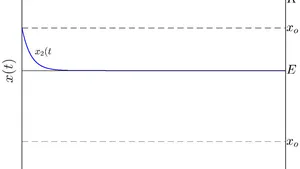
As shown in the appendix, if we have that a - b < 0, then for , the global trajectory acquires the form given by Equation (13) with . Therefore, is monotonically decreasing for all . Because of this, the population size vanishes according to an exponential law. Alternatively, if a < b and , will initially conform to the branch given by Equation (14), setting . Since a < b implies K < E, we have and asymptotically approaching the value K. But, by continuity on its descent towards K, there necessarily will be a time such that . Afterwards, the dynamics will follow the split, which because of the ordering a < b, will drive population size to vanish. We can summarise that maintenance of the condition a < b implies the disappearance of the population, regardless of its initial value (also regardless of whether this value is greater or equal or less than E, see Figure 1).
{"image_source":{"path":"images/54547f099811db9d572419c528d27e5efde2623a67a9c0653eaf23299bf03bcf.jpg"},"content":"","chart_caption":[{"type":"text","content":"Figure 1: The behaviour of the trajectory "},{"type":"equation_inline","content":"x(t)"},{"type":"text","content":" for a < b. For "},{"type":"equationinline","content":"x{0} \leq E"},{"type":"text","content":", population size "},{"type":"equation_inline","content":"x(t)"},{"type":"text","content":" vanishes, following an exponential law, provided that a < b. Whenever a < b and "},{"type":"equationinline","content":"x{0} > E"},{"type":"text","content":", population size "},{"type":"equation_inline","content":"x(t)"},{"type":"text","content":" decreases initially according to the "},{"type":"equationinline","content":"x{2}(t)"},{"type":"text","content":" correspondence rule approaching the asymptotic value K, which lies below E, when crossing this threshold, the trajectory "},{"type":"equation_inline","content":"x(t)"},{"type":"text","content":" ceases to behave according to the rule "},{"type":"equationinline","content":"x{2}(t)"},{"type":"text","content":" and switches to the "},{"type":"equationinline","content":"x{1}(t)"},{"type":"text","content":" path, and therefore, asymptotically approaching zero as t progresses to infinity."}],"chart_footnote":[]}
Consider now the a > b order. Then, we will also have K > E. Then, for , at the beginning of the growth process, population size will describe according to the exponentially increasing path . Furthermore, since by continuity, there will be a time such that . Afterwards, the dynamics will switch to being modelled by the stem. Therefore, as the appendix explains, population size will keep increasing and asymptotically approaching K > E. The case a > b and portraits similarly with behaving as the branch and asymptotically approaching K. Besides, whenever a > b and , the population size will be described by , so the condition will fix to be decreasing and asymptotically approaching Kas t progresses to infinity (Figure 2).
{"image_source":{"path":"images/f6a1327befddb9713a8452e4afb289425f0c2d424414f07df7c94b8455214818.jpg"},"content":"","chart_caption":[{"type":"text","content":"a"},{"type":"text","content":"Figure 2: The behaviour of the "},{"type":"equation_inline","content":"x(t)"},{"type":"text","content":" trajectory for "},{"type":"equation_inline","content":"a > b"},{"type":"text","content":". For "},{"type":"equation_inline","content":"a > b"},{"type":"text","content":" and "},{"type":"equation_inline","content":"x_0 \leq E < K"},{"type":"text","content":", at the beginning of the process, population size "},{"type":"equation_inline","content":"x(t)"},{"type":"text","content":" increases according to the "},{"type":"equation_inline","content":"x_1(t)"},{"type":"text","content":" branch; because of continuity, "},{"type":"equation_inline","content":"x_1(t)"},{"type":"text","content":" will reach the "},{"type":"equation_inline","content":"E"},{"type":"text","content":" threshold at a time "},{"type":"equation_inline","content":"t_c"},{"type":"text","content":". For "},{"type":"equation_inline","content":"t \geq t_c"},{"type":"text","content":", population size will keep growing according to "},{"type":"equation_inline","content":"x_2(t)"},{"type":"text","content":", thereby asymptotically approaching level "},{"type":"equation_inline","content":"K"},{"type":"text","content":". The case "},{"type":"equation_inline","content":"a > b"},{"type":"text","content":" and "},{"type":"equation_inline","content":"E < x_0 < K"},{"type":"text","content":" renders similarly with "},{"type":"equation_inline","content":"x(t)"},{"type":"text","content":" behaving as the "},{"type":"equation_inline","content":"x_2(t)"},{"type":"text","content":" branch approaching "},{"type":"equation_inline","content":"K"},{"type":"text","content":". For "},{"type":"equation_inline","content":"a > b"},{"type":"text","content":" and "},{"type":"equation_inline","content":"x_0 > K"},{"type":"text","content":", the trajectory decreases from "},{"type":"equation_inline","content":"x_0"},{"type":"text","content":" and approaches the equilibrium level "},{"type":"equation_inline","content":"K"},{"type":"text","content":"."}],"chartfootnote":[]} For a = b and the $x{0} \leq E$ ordering, population size determines by , so it remains stationary at . Assuming that the arrangement a = b and holds, at the start of the growing process, the trajectory will be determined by the rule with the initial condition . As the appendix explains, we also have for this parameter arrangement so the trajectory shall decrease and asymptotically approach E.
{"image_source":{"path":"images/3d16f52949aa88a587a61afbd94fb341a7021c63fc5f93728dcea8c715cbd083.jpg"},"content":"","chart_caption":[{"type":"text","content":"Figure 3: The behaviour of the "},{"type":"equation_inline","content":"x(t)"},{"type":"text","content":" trajectory for "},{"type":"equation_inline","content":"a = b"},{"type":"text","content":". For "},{"type":"equation_inline","content":"x_0 \leq E"},{"type":"text","content":" and "},{"type":"equation_inline","content":"a = b"},{"type":"text","content":", the "},{"type":"equation_inline","content":"x(t)"},{"type":"text","content":" trajectory remains stationary. For "},{"type":"equation_inline","content":"a = b"},{"type":"text","content":" and "},{"type":"equation_inline","content":"x_0 > E"},{"type":"text","content":", the trajectory "},{"type":"equation_inline","content":"x(t)"},{"type":"text","content":" decreases and asymptotically approaches "},{"type":"equation_inline","content":"E"},{"type":"text","content":"."}],"chartfootnote":[]} In summary, the case a = b entitles a heterogeneous behaviour because if the magnitude of the initial population satisfies $x{0} < E$, then population size remains steady. However, if the initial population size lies above the E threshold, i.e. , then decreases and asymptotically approaches the E threshold (Figure 3).
3.2 Fitting Results
In what follows, we explain the performance of LLPM, Liebig's law population model of Equation (9), as an exploratory tool given different data sets. We address data on yeast grown under ideal conditions in a test tube and the growth of a harbour seal population, both reported by Avissar et al. (2013). We also consider data reported by R. Pearl on the growth of Drosophila melanogaster (Pearl, 1927) and data reported by Hughes and Tanner (2000) on the slow decline of an Agaricia agaricites population on Jamaican reefs. Fitted parameters, associating standard deviations and Concordance Correlation Coefficient (CCC) values, also denoted utilising the symbol (Lin, 1989), appear in Table 1. To compare the reproducibility strength of offered LLPM, we include CCC values of fits of the logistic model of Equation (19) performed on the included data sets.
Table 1: Estimated values of initial population and resource sizes and , as well as parameter, values and produced by fitting the LLVM of Equation (9) to the listed data sets (Avissar et al., 2013; Pearl, 1927; Hughes & Tanner, 2000). Concordance Correlation Coefficient ( ) values are also displayed. LLPM stands for CCC value linking to the LLPM of Equation (9), LOGdenotes CCC produced by a fit of the logistic model of Equation (19).
| Data set | $x_o$ | a | b | E | $R_0$ | K | p | ρLLPM | ρLOG |
| Yeast | 1.1 | 0.2549 | 0.0452 | 5.7925 | 8.1388 | 12.827 | 0.5 | 99.23% | 98.19% |
| Seal | 1634.24 | 0.3142 | 0.1748 | 4345.66 | 4350 | 7801 | 0.0016 | 92.97% | 86.91% |
| Fruit fly | 13.0039 | 0.4956 | 0.3616 | 235 | 279.39 | 303.31 | 0.2 | 99.43% | 99.43% |
| Coral | 142.62 | 0.1070 | 0.2565 | 376.49 | 376.871 | 157.20 | 0.0016 | 91.43% | 88.99% |
We first considered data on yeast growing under ideal conditions in a test tube portrayed in Figure 45.10a) in Avissar et al. (2013) and reproduced here in Figure 4a. We know that the yeast growth curve shown in Panel (a), as portrayed in Avissar et al. (2013), suggests an inconsistent placement of the initial condition . Nevertheless, blue lines in Figure 4b display a consistent S-shaped curve fitted by the logistic model of Equation (19) on yeast data ( , , , ). Afterwards, we produced a fit of Liebig's law of the minimum-driven model of Equation (9) (LLPM) to yeast data. Fitted LLPM parameters values were , , , and , which through Equations (10) and (11) produced and one to one. Concurring reproducibility index value was . Comparing the shapes of the trajectories of the yeast population displayed in Figure 4, we can be aware that blue lines fitted by the present LLPM (Panel c) consistently describe an S-shaped pattern. Panel (c) also shows the shape of the fitted form of the resource abatement function as given by Equation (3) (red lines). Avissar et al. (2013) do not refer to whatever energy source the yeast population depended on, but in any event, the shape of the fitted form of suggests that independently of bulk consumption, the yeast population and its feeding resource stabilised one to one.
{"image_source":{"path":"images/d30c7d40aa56b6a4148cfe3c43914c0bbbf9f15df4cad3a4a03e8ff989b37347.jpg"},"content":"","chart_caption":[],"chart_footnote":[]} {"image_source":{"path":"images/8b5c1c0d501063cfbf803d40fe0f6f6b18d6c93b95fc6db471e186369a250c2e.jpg"},"content":"","chart_caption":[],"chart_footnote":[]}
{"image_source":{"path":"images/9bd5371742c7021d4d6bc17e9da249ab9cf61ebee20f5cc3681229cf70ccc081.jpg"},"content":"","chart_caption":[{"type":"text","content":"Figure 4: Yeast growth data from Avissar et al. (2013). Panel (a) is an assumed S-shaped logistic growth curve pattern associated with yeast grown under ideal conditions in a test tube, as in"}],"chart_footnote":[]}
Figure 45.10a in Avissar et al. (2013). Panel (b) displays a fit of the logistic model as given by Equation (19) to referred yeast data (blue lines). Panel (c) exhibits the spread of observed data points about the trajectory resulting by fitting LLPM, Liebig's law of the minimum-driven model of Equation (9), to the yeast growth data adapted from Panel (a) (blue lines). Panel (c) also shows the shape of the fitted form of the resource abatement function as given by Equation (3) (red lines).
Figure 5a presents the harbour seal populationdata in Figure 45.10b in Avissar et al. (2013). Figure 5b presents the spread of referred seal data about the logistic curve fitted by the model of Equation (19). Concordance Correlation Coefficient resulted in a value of , and parameter estimates were , , . Figure 5c shows the spread of captured seal data about the trajectory produced by a fit of LLPM, Liebig's law of the minimum-based model of Equation (9). Corresponding fitted parameters values were , , , , and , which employing equations (10) and (11) produced and one to one. The reproducibility index acquired a value of . The associating form of (red lines in Panel (c) suggests that the steady form of the LLPM given by Equation (15) also fits consistently. This fact explains by the small fitted value for the parameter . Moreover, Panel (d) displays a close-up look at the variation of , corroborating that this function remained close to its initial value independently of consumption by the seal population.
{"image_source":{"path":"images/35fcdce4201aef305330564f990572cc53e08cddc3026b152a48b7ee789c8471.jpg"},"content":"","chart_caption":[],"chart_footnote":[]} {"image_source":{"path":"images/5841ef2f7c659ecf10379da6cdb522fee90ca5d2e52bf6ef99d32475721aebce.jpg"},"content":"","chart_caption":[{"type":"text","content":"b"}],"chart_footnote":[]}
{"image_source":{"path":"images/8339dbce3ab49ed646da1033f80854ed6fef3f1d00f83881675449cad57ef9b5.jpg"},"content":"","chart_caption":[{"type":"text","content":"c"}],"chart_footnote":[]} {"image_source":{"path":"images/9dad6ee5824e909448010d3ea773525ef03ec29da6773b5d0e8781533c78559c.jpg"},"content":"","chart_caption":[{"type":"text","content":"d"},{"type":"text","content":"Figure 5: Fit of the LLPM on seal population growth data as reported in Avissar et al. (2013). Panel (a) is a presumed logistic growth curve pattern associated with a harbour seal population, as portrayed in Figure 45.10b in Avissar et al. (2013). Panel (b) exhibits the spread of the Avissar et al. (2013) harbour seal data about curves fitted by the conventional logistic model of Equation"}],"chart_footnote":[]}
(19). Panel (c) shows data spread about the trajectory resulting by fitting LLPM Liebig's law of the minimum-driven model of Equation (9) to the available seal population growth data—panel (d) variation of the fitted resource availability function .
Correspondingly, Figure 6a presents the spread of data reported by R. Pearl on the growth of Drosophila melanogaster (Pearl, 1927) about the logistic curve fitted by the model of Equation (19). Fitted parameter values were a = 6.19, K = 329.7, and with Concordance Correlation Coefficient at a value of . Figure 6b shows the spread of captured Drosophila melanogaster data about the trajectory produced by a fit of LLPM, Liebig's law of the minimum-based model of Equation (9). Fitted parameters values were a = 0.4956, b = 0.3616, , , p = 0.2, which through Equations (10) and (11) produced E = 235 and K = 303.31 one to one. Red lines on panel b display the variation of feeding resource availability , showing that although population consumption induced an asymptotical approach to a value K, resource abatement was moderate.
{"image_source":{"path":"images/fe43367f1d8b5055066cdc38783ceec6d6a1f4511d01c6fad0212163c72f635f.jpg"},"content":"","chart_caption":[],"chart_footnote":[]} {"image_source":{"path":"images/15c891b6ca9c5ae4b38b6abd2dc28902bc922c7fbeb38df947d7f60dba6e3cbc.jpg"},"content":"","chart_caption":[{"type":"text","content":"b"},{"type":"text","content":"Figure 6: Fit of LLPM on Drosophila melanogastergrowth data presented in Pearl (1927). Panel (a) displays a fit of the logistic model as given by Equation (19) to Drosophila melanogaster data, with Panel (b) exhibits the spread about the "},{"type":"equation_inline","content":"x(t)"},{"type":"text","content":" trajectory resulting by fitting the Liebig's law of the minimum-driven model of Equation (9) to Drosophila melanogaster data. This last Panel also shows the shape of the fit of the resource abatement function "},{"type":"equation_inline","content":"R(t)"},{"type":"text","content":" as given by Equation (3)."}],"chart_footnote":[]}
Finally, Figure 7a presents the spread of data reported by Hughes and Tanner (2000) on the decline of an Agaricia agaricites population on Jamaican reefs about the logistic curve fitted by the model of Equation (19) with , , and a Concordance Correlation Coefficient of . This fit identified the declining branch of the logistic model. However, it resulted in incompatibly negative values for the parameters and . Figure 7b shows the spread of captured Agaricia agaricites data about the trajectory produced by a fit of Liebig's law of the minimum-based model of Equation (9). Fitted parameters values were , , , , , which employing
Equations (10) and (11) produced E = 376.49 and K = 157.20, one to one. Compared to an unreliable fit of the logistic model shown in Panel b), an LLVM try predicts the extinction of the Agariciaagaricites population. In coherence, the LLVM predicts that the feeding resource path adapts to a steadily growing pace of stabilisation (panel c). Then regardless of plentiful feeding energy, the Agaricia agaricites population vanished away.
{"image_source":{"path":"images/b104ed2f13374376d0fd5a5cd7a3522f51a9c093b668f766c4e32c8e26c4f068.jpg"},"content":"","chart_caption":[],"chart_footnote":[]} {"image_source":{"path":"images/f2c50995376a07434826013b70b5eeb655ed7d79edc1103dfcd87ab95e2a9b1c.jpg"},"content":"","chart_caption":[],"chart_footnote":[]}
{"image_source":{"path":"images/494fa8e1accb1072352a893433936e93df49b1ec1176abf53f7a5cb361719188.jpg"},"content":"","chart_caption":[{"type":"text","content":"Figure 7: Fitting results of the LLPM on Agaricia agaricites growth data presented in Hughes and Tanner (2000). Panel (a) displays a fit of the logistic model given by Equation (19) to Agaricia agaricites data. Panel (b) exhibits the spread about the "},{"type":"equation_inline","content":"x(t)"},{"type":"text","content":" trajectory resulting by fitting Liebig's law of the minimum-driven model of Equation (9) to Agaricia agaricites data and also shows the shape of fitted form of the resource abatement function "},{"type":"equation_inline","content":"R(t)"},{"type":"text","content":" as given by Equation (3). Panel(c) close-up at the "},{"type":"equation_inline","content":"R(t)"},{"type":"text","content":" variation."}],"chart_footnote":[]}
IV. DISCUSSION
In cellular structures such as mitochondria, the maxima or minima of a periodical chemical reaction proved to be determinants of observable patterns (Woodcock, 1978). In other processes, for instance, catalysis, limiting values of variables such as pH and temperature can cause enzymes to lose their functionality, thereby impairing the easing of essential chemical reactions within living organisms (Dyson & Noltmann, 1968). Besides, the maximum and minimum blood glucose levels, body temperature, or pH range are critical for maintaining homeostasis (Yildiz et al., 2020). Furthermore, maximum and minimum values can activate regulatory mechanisms in biological systems that help organisms deal with and adapt to challenging environmental conditions. Within these response mechanisms, we can include activation of heat shock proteins that shield cells from harm given extreme values of temperature or water conservation mechanisms in plants in response to extreme osmotic conditions (Bich et al., 2016; Sharp et al., 1999; Chaves & Oliveira, 2004). Another example of extreme value control of a biological process is the existence of a minimum light intensity needed for efficient photosynthesis in plants (Boardman, 1977; Madsen & Sand-Jensen, 1994). What is more, in this vein, it is worth mentioning that extreme levels of light intensity or CO2 concentrations can restrict the effectiveness of photosynthesis and, as a result, hamper the capability of plants to create energy (Jolliffe & Tregunna, 1968). Therefore, from a general perspective, comprehending the upper and lower limits of biologically relevant variables delivers an understanding of organisms' underlying limits, adaptive responses, and constraints.
In ecological settings, extreme values are often more descriptive of relevant dynamics than standard measures of central tendency (Gaines & Denny, 1993; Montiel et al., 2004). Issues relating to physical stress, such as high or low temperatures, salinity, soil water content, wind velocities, and varying durations of air exposure, serve as examples (Denny & Deines, 1990). Moreover, characterising extreme values not only aids in defining the optimal operational boundaries for ecological processes and contributes to our interpretation of the correlation between organisms and their environment (Ruthsatz, Dausmann, and Peck, 2022). For instance, species interaction dynamics and community formation depend on the maximum and minimum values of different variables (Checa et al., 2014). Furthermore, the availability of particular resources can limit the distribution of species or the sizes of their populations (Wright, 1983), while the sizes of predator populations below or above given edges can impact the distribution and behaviour of prey species (Schneider, 2001). Also, from an ecological perspective, acknowledging the relevance of maximum and minimum values of pertinent variables contributed to conceiving the concept of tolerance bounds (Niinemets & Valladares, 2008; Pörtner, 2001; Goss & Bunting, 1976). For example, the minimum oxygen concentration required for aquatic organisms' survival sets their tolerance lower limit (Seibel, 2011; Gaufin et al., 1974). Likewise, the maximum temperature at which an organism can survive or reproduce entails its thermal tolerance upper limit (Madeira et al., 2012; Buckley & Huey, 2016). Ecological niches, characterised by certain variables' upper and lower limits, determine a species' optimal environmental conditions (Galparsoro et al., 2009). Therefore, including maximum and minimum thresholds for factors such as temperature, moisture, or nutrient availability helps to understand how organisms distribute and their ecological requirements (Kearney, 2006). Moreover, the notion of extreme value control significantly contributed to conceiving important theoretical constructs in ecological research, such as the Principle of Limiting Factors, developed based on results reported by Justus Von Liebig in 1843 (Liebig, 1843), the Law of Tolerance conceived by Victor Ernest Shelford in the early 20th century. Moreover, the Theory of the Niche, first proposed by the ecologist G. Evelyn Hutchinson in 1957, states that each species has a range of environmental conditions in which it can thrive (Hutchinson, 1957; Hutchinson, 1978; Polechová & Storch, 2008).
In summarising the passage above, it is worth emphasising that to understand better the underlying limits, changes, and necessities of living organisms; it is essential to determine the upper and lower limits that set the intervals of influence of their determining physical and biological variables. This understanding of suitable extreme values assists in setting the boundaries that biological processes must function within, leading to a better comprehension of how organisms work in conjunction with their surroundings to function efficiently. Notwithstanding, when referring to conceiving constructs aimed to model population dynamics, besides a reduced number of papers (e.g. Polyetayev, 1971; Echavarria & Gomez, 1979; Echavarria-Heras et al. 2021 Montiel-Arzate et al. 2004; Echavarria-Heras et al., 2021) the relevance of including extreme values of causal variables in a dynamical set up has not been adequately acknowledged in the literature. For that reason, we decided to further contribute to the matter, so, in this work, we modified the protocol by Echavarria-Heras et al. (2021) that resulted in the construct given by Equation (9), which we refer to as LLPM, for a single species population growth model, built upon Liebig's Principle of Limiting Factors. The LLPM sustains by hypothesising that: (1) the inherent natural natality rate is determined according to Liebig's Law by the minimum between the size of the population and that of its feeding resource, , at a time , (2) the accompanying natural mortality rate is supposed to be proportional solely to population size, and (3) the rate of consumption of the external feeding resource ostensibly varies directly proportional to the natural growth rate of the population. Despite being partially founded on the assumption that mortality depends linearly on population size, the qualitative exploration of the behaviour of the global trajectory associated with the offered LLPM demonstrated a proven capability to mimic the typical s-shaped pattern associated with restricted growth models. The presented fitting results confer the LLPM of excellent reproducibility features and reveal that such a paradigm offers a remarkable interpretative strength. Firstly, the LLPM could identify the suggested form for the resource abatement function on the fly, entailing a feature that the typical logistic growth model of Equation (19) lacks. Secondly, also compared to the presently addressed logistic model, the LLPM offers a consistent way to identify a declining pace in population size leading to extinction which the latter model could not suitably achieve. Besides, simplifying complexity has been proven advantageous in finding parameter estimates for consistent reproducibility of real data sets.
Nevertheless, performing research on further simplifying the nonlinear parameter estimation tasks deems necessary.
V. APPENDIX. ANALYTICAL APPROACH
5.1 Continuity property of the global trajectory
Equation (12) states that the global trajectory , associating to the piecewise-defined ODE given by Equation (9), expresses such that
where agreeing to Equations (10) and (11), we have
and
with p, as explained around Equation (3), stands for the constant of proportionality between the resource consumption and natural population growth rates.
The constants and values in Equation (A1) follow from the requirement that along with the continuity condition , being a time value such that . The value of is determined depending on the ordering relationships between a and b, along with the placement of the initial condition relative to the E threshold. Two ordering arrangements prompt the global trajectory to cross the E threshold. The first one involves a>b and , and another composing a<b and .
5.2 Continuity of the global trajectory in the case a > b and
Assume that we have a > b and . Then, at the beginning of the growth process, the global trajectory shapes according to the branch holding in the domain and given by Equation (A1). Then to accomplish the suitable form , we must choose ; that is, we acquire
According to Equation (A1), the complementary branch of the global trajectory , holding in the domain , depends on the initial condition , whose value ought to be determined. For that aim, we must enforce that the global trajectory is continuous at a time such that or equivalently and . Therefore, we first need to obtain . For achieving that task, we rely on the statement , so, using Equation (A2), we must have
from which solving for yields
Secondly, we need to consider that continuity of at fulfils if and only if also satisfies . Agreeing with Equation (A1), this statement requires adapting a suitable value of the initial condition , which makes
Then, solving for , we obtain
Moreover, equivalently replacing , as given by Equation (A3), one gets
Being identified, we can obtain the form of the branch joining the initial one to compose the global trajectory .
5.3 Continuity of global trajectory in the case a < b and
In turn, for a < b and , agreeing to Equation (A1), the first portion of the global trajectory , turns out to be
Then, to complete the path , we need to get the complementary portion holding in the domain . As stated by Equation (A1) requires adapting the value of the associating initial condition such that the property that is continuous at a time for which succeeds. Again, this entails both and taking a common value . From Equation (A6), the statement leads to
which in turn, allows solving for namely
Correspondingly, using Equation (A1) to express the condition , then solving for yields
from which, after replacing as given by (A7), leads to
5.4 Construction of the global trajectory for the case a < b
Whenever and , initially the dynamics sets by as given by Equation (A2) namely
Then, is decreasing for all . Therefore, for . Consequently, the global trajectory maintains the shape for . Besides, we have
Because of this, the population size vanishes according to an exponential law.
Assume now that a < b and . Then, initially, will conform to as given by Equation (A6), that is,
Since by assumption a < b and we also have E > 0, it follows that,
Since as it is stated by Equation (A1), we have , inequality (A10) along the statement, yield the ordering,
On the other hand, from Equation (A6), the derivative of becomes.
Since for , the sign of shall be fixed by the factor . Then, since inequality (A11) holds, we have , which implies . Hence, for a < b and , we have established that becomes a decreasing function of time t. On the other hand, from Equation (A6), we also have that
Therefore, the path bears a horizontal asymptote K. Note also that because a < b, by inequality (A11), we also have K < E. Therefore, the limiting value of whenever will lie below E. Then, necessarily the trajectory keeps on decreasing until it reaches the value E, that is, there exists a time value as given by Equation (A7) such that and after that, the dynamics of will set by , that according to Equation (A1) bears a form
Then, choosing
adds the continuity condition , as much as setting to decrease asymptotically towards zero (see Figure A1b).
We can summarise what we have explored so far by stating that maintenance of the condition a < b implies the disappearance of the population, regardless of its initial value (also regardless of whether this value is greater or equal or less than E).
{"image_source":{"path":"images/bdfd806e105370411efdaa7364a4c4488c3127cfe6ddceee17aebdf295f969ac.jpg"},"content":"","chart_caption":[],"chart_footnote":[]} {"image_source":{"path":"images/c6b51597a0033e53f213bc153dc50c469fcfff68a37764728edacd1853d4dd2e.jpg"},"content":"","chart_caption":[{"type":"text","content":"Figure A1: Construction of the "},{"type":"equation_inline","content":"x(t)"},{"type":"text","content":" trajectory for a < b. Provided a < b, then for "},{"type":"equationinline","content":"x{0} \leq E"},{"type":"text","content":", the population size "},{"type":"equation_inline","content":"x(t)"},{"type":"text","content":" vanishes following the exponential law "},{"type":"equationinline","content":"x{1}(t)"},{"type":"text","content":" given by Equation (A1) with "},{"type":"equationinline","content":"x{10} = x_{0}"},{"type":"text","content":" (Panel a). For a < b and "},{"type":"equationinline","content":"x{0} > E"},{"type":"text","content":", initially "},{"type":"equation_inline","content":"x(t)"},{"type":"text","content":" takes on an "},{"type":"equationinline","content":"x{2}(t)"},{"type":"text","content":" form given by Equation (A1), which decreases asymptotically to a value K < E. When crossing the horizontal line x = E, at a time "},{"type":"equationinline","content":"t{c}"},{"type":"text","content":", the trajectory "},{"type":"equation_inline","content":"x(t)"},{"type":"text","content":" ceases to be given by "},{"type":"equationinline","content":"x{2}(t)"},{"type":"text","content":" that would take it to the limit value K by t approaching infinity and begins following an "},{"type":"equationinline","content":"x{1}(t)"},{"type":"text","content":" shaped trajectory with "},{"type":"equationinline","content":"x{10} = E e^{(-(a-b)t_{c})}"},{"type":"text","content":". Therefore, "},{"type":"equation_inline","content":"x(t)"},{"type":"text","content":" will asymptotically progress to zero as t approaches infinity."}],"chart_footnote":[]}
5.5 Construction of the trajectory for the case a > b
Now suppose that inequality a > b fulfils. Then, E > 0 implies
Now, since Equation (A1) establishes, , inequality above implies the ordering
Suppose that a - b > 0 and . Under these conditions, as specified by inequality (A14), we also have the K > E order. And, as given by Equation (A2), at the beginning of the process, the population size will be set by
Then, once it departs from , will increase exponentially. And, since , as we elaborated around Equation (A3) by continuity of the global trajectory , there will be a time satisfying,
at which population , as given by , will meet the Ethreshold, that is, . For , according to Equation (A1), population size will switch from the growth form to one. Again, Equation (A12) states that the sign of sets by the factor . Then, will increase whenever , and as stated by Equation (A13), approaches K as t progresses to infinity (Figure A2a).
Assume that in addition to a > b, the initial condition places such that . Under these circumstances, the process will be conducted for a certain initial period by the branch of the trajectory , as established by Equation (A6). Again, Equation (A12) states that the sign of shall fix by the factor . Then, will increase whenever , and as stated by Equation (A13), approaches K as t progresses to infinity (Figure A2a). Besides, whenever a > b and , the population size will be described by , attaining a form given by Equation (6), that is,
Then, as we have elaborated above, the condition sets the branch of the global trajectory to be decreasing and asymptotically approaching K as t progresses to infinity (Figure A2b).
{"image_source":{"path":"images/2e1ac80f1a5858552b78906ee01c53631ba0a91eea5e808445ee5b2bc39ec991.jpg"},"content":"","chart_caption":[],"chart_footnote":[]} {"image_source":{"path":"images/359aa42d98699bb0aa181d42b80df51eebef8c29d4a6df0110c5c7df7d8b9764.jpg"},"content":"","chart_caption":[{"type":"text","content":"Figure A2: Construction of the "},{"type":"equation_inline","content":"x(t)"},{"type":"text","content":" trajectory for a > b. Whenever a > b and "},{"type":"equationinline","content":"x{0} \leq E"},{"type":"text","content":" at the beginning of the process, population size "},{"type":"equation_inline","content":"x(t)"},{"type":"text","content":" will be ruled by "},{"type":"equationinline","content":"x{1}(t)"},{"type":"text","content":" as given by Equation (9), and consequently, it will increase. By continuity, "},{"type":"equationinline","content":"x{1}(t)"},{"type":"text","content":" will eventually reach the E threshold, and the dynamics will start to be modelled by the "},{"type":"equationinline","content":"x{2}(t)"},{"type":"text","content":" branch of the global trajectory "},{"type":"equation_inline","content":"x(t)"},{"type":"text","content":", thereby approaching the equilibrium level K when t progresses to infinity. The case a > b and "},{"type":"equationinline","content":"E < x{0} < K"},{"type":"text","content":" portraits similarly with "},{"type":"equation_inline","content":"x(t)"},{"type":"text","content":" behaving as the "},{"type":"equationinline","content":"x{2}(t)"},{"type":"text","content":" branch and asymptotically approaching K (Panel a). Besides, whenever a > b and "},{"type":"equationinline","content":"x{0} > K > E"},{"type":"text","content":", the population size "},{"type":"equation_inline","content":"x(t)"},{"type":"text","content":" will be described by "},{"type":"equationinline","content":"x{2}(t)"},{"type":"text","content":", so the condition "},{"type":"equationinline","content":"x{0} > K"},{"type":"text","content":" will fix "},{"type":"equation_inline","content":"x(t)"},{"type":"text","content":" to be decreasing and asymptotically approaching K as t progresses to infinity (Panel b)."}],"chart_footnote":[]}
Summarising, whenever a > b, then either the, or placements of the initial condition will drive the population size being monotonically increasing and approaching K. If instead , will be monotonically decreasing with K as an asymptote. As a consequence of this, could stand as a specific equilibrium state of the system determined by a and b, the internal development processes that set the intensities of the natality and mortality processes , as well as, by the external factor E.
5.6 Analysis of case a = b
Let us now analyse the behaviour of for the case a = b. Again comparing and E, we may first consider the order. As we already know, for this case, the behaviour of the trajectory is determined by the branch as given by Equation (A2), namely . Then, since by assumption a = b, we have . The trajectory remains stationary (Figure A3a).
For a = b and , the trajectory follows the rule at the start of the growing process. According to Equation (A6) for a = b, becomes,
Then we have
Equation (A15) yields
Nevertheless, since we established the condition , then so the trajectory shall be decreasing and asymptotically approaching E as tprogresses to infinity (Figure A3b).
In short, the case a = b entitles a heterogeneous behaviour because if the magnitude of the initial population satisfies , then population size remains steady. However, if the initial population size lies above the E threshold, i.e. , then decreases exponentially and asymptotically approaches the equilibrium level E.
{"image_source":{"path":"images/3eddc7f9c6cdde8f8bc72e4895e24339d2ab0d1f0931542d485abbe2f3083c55.jpg"},"content":"","chart_caption":[],"chart_footnote":[]} {"image_source":{"path":"images/562c523afc1bdd410d0bb64b914d0f695a87db24e8cc58073cb94c906cd250ad.jpg"},"content":"","chart_caption":[{"type":"text","content":"Figure A3: The shape of "},{"type":"equation_inline","content":"x(t)"},{"type":"text","content":" for a = b. For a = b and "},{"type":"equationinline","content":"x{0} \leq E"},{"type":"text","content":", the "},{"type":"equation_inline","content":"x(t)"},{"type":"text","content":" trajectory remains stationary (Panel a). If the initial population size lies above the E threshold, i.e. "},{"type":"equationinline","content":"x{0} > E"},{"type":"text","content":", then "},{"type":"equation_inline","content":"x(t)"},{"type":"text","content":" decreases exponentially and asymptotically approaches E."}],"chart_footnote":[]}
Summarising, the case a = b entitles a heterogeneous behaviour because if the magnitude of the initial population satisfies , then population size remains steady. However, if the initial population size lies above the E threshold, i.e. , then decreases and asymptotically approaches the E threshold.
ACKNOWLEDGEMENTS
The authors would like to thank CICESE, our honorable and generous institution that this year celebrates its 50th anniversary and whose unrestricted support has allowed our consolidation as scientists. Hector Echavarria Heras expresses special thanks to Guillermo Gómez Alcaraz for suggesting pursuing this research. We also thank three anonymous reviewers for their valuable and enlightening comments.
Conflict of Interest
The authors declare no conflict of interest.
Ethical Approval
Not applicable
Data Availability
The datasets used in this study are openly available at [repository link] and the source code is available on GitHub at [GitHub link].
Funding
This work did not receive any external funding.
References
Cite this article
Related Research



Special Issue
Launch a focused special issue to highlight research, emerging trends, and expert insights in your academic field.
